The zoo of neural network types grows exponentially. One needs a map to navigate between many emerging architectures and approaches.
Fortunately, Fjodor van Veen from Asimov institute compiled a wonderful cheatsheet on NN topologies. If you are not new to Machine Learning, you should have seen it before:
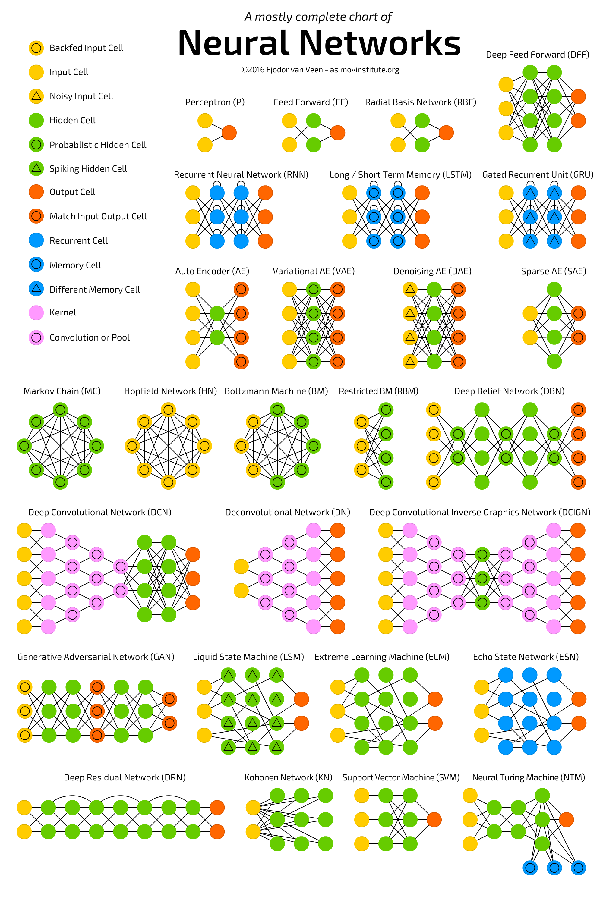
In this story, I will go through every mentioned topology and try to explain how it works and where it is used. Ready? Let’s go!
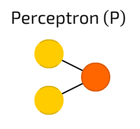
Perceptron. The simplest and oldest model of Neuron, as we know it. Takes some inputs, sums them up, applies activation function and passes them to output layer. No magic here.
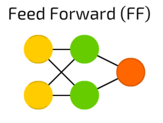
Feed forward neural networksare also quite old — the approach originates from 50s. The way it works is described in one of my previous articles — “The old school matrix NN”, but generally it follows the following rules:
- all nodes are fully connected
- activation flows from input layer to output, without back loops
- there is one layer between input and output (hidden layer)
In most cases this type of networks is trained using Backpropagation method.
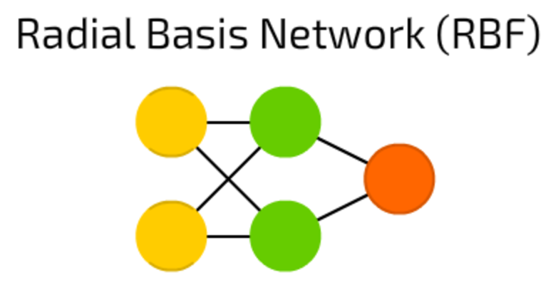
RBF neural networks are actually FF (feed forward) NNs, that use radial basis function as activation function instead of logistic function. What makes the difference?
Logistic function map some arbitrary value to a 0…1 range, answering a “yes or no” question. It is good for classification and decision making systems, but works bad for continuous values.
Contrary, radial basis functions answer the question “how far are we from the target”? This is perfect for function approximation, and machine control (as a replacement of PID controllers, for example).
To be short, these are just FF networks with different activation function and appliance.
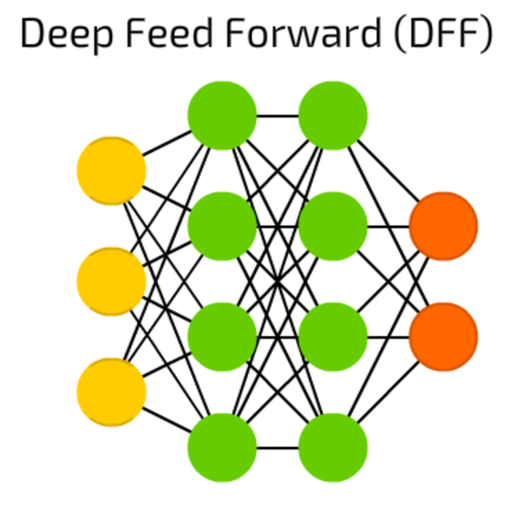
DFF neural networks opened pandora box of deep learning in early 90s. These are just FF NNs, but with more than one hidden layer. So, what makes them so different?
If you read my previous articleon backpropagation, you may have noticed that, when training a traditional FF, we pass only a small amount of error to previous layer. Because of that stacking more layers led to exponential growth of training times, making DFFs quite impractical. Only in early 00s we developed a bunch of approaches that allowed to train DFFs effectively; now they form a core of modern Machine Learning systems, covering the same purposes as FFs, but with much better results.
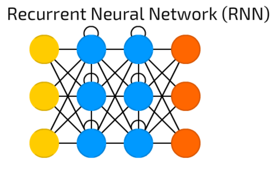
Recurrent Neural Networksintroduce different type of cells — Recurrent cells. The first network of this type was so called Jordan network, when each of hidden cell received it’s own output with fixed delay — one or more iterations. Apart from that, it was like common FNN.
Of course, there are many variations — like passing the state to input nodes, variable delays, etc, but the main idea remains the same. This type of NNs is mainly used then context is important — when decisions from past iterations or samples can influence current ones. The most common examples of such contexts are texts — a word can be analysed only in context of previous words or sentences.

This type introduces a memory cell, a special cell that can process data when data have time gaps (or lags). RNNs can process texts by “keeping in mind” ten previous words, and LSTM networks can process video frame “keeping in mind” something that happened many frames ago. LSTM networks are also widely used for writing and speech recognition.
Memory cells are actually composed of a couple of elements — called gates, that are recurrent and control how information is being remembered and forgotten. The structure is well seen in the wikipedia illustration (note that there are no activation functions between blocks):
The (x) thingies on the graph are gates, and they have they own weights and sometimes activation functions. On each sample they decide whether to pass the data forward, erase memory and so on — you can read a quite more detailed explanation here. Input gate decides how many information from last sample will be kept in memory; output gate regulate the amount of data passed to next layer, and forget gates control the tearing rate of memory stored.
This is, however, a very simple implementation of LSTM cells, many others architectures exist.
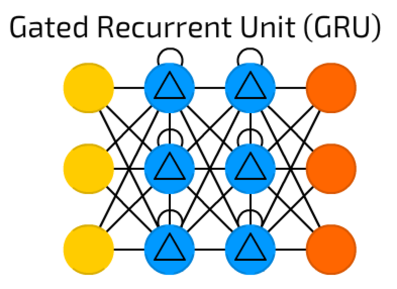
GRUs are LSTMs with different gating. Period.
Sounds simple, but lack of output gate makes it easier to repeat the same output for a concrete input multiple times, and are currently used the most in sound (music) and speech synthesis.
The actual composition, though, is a bit different: all LSTM gates are combined into so-called update gate, and reset gate is closely tied to input.
They are less resource consuming than LSTMs and almost the same effective.
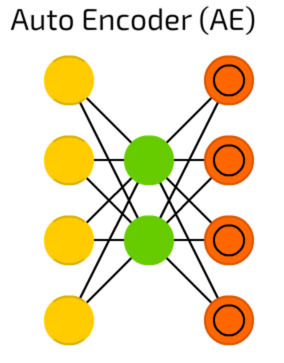
Autoencoders are used for classification, clustering and feature compression.
When you train FF neural networks for classification you mostly must feed then X examples in Y categories, and expect one of Y output cells to be activated. This is called “supervised learning”.
AEs, on the other hand, can be trained without supervision. Their structure — when number of hidden cells is smaller than number of input cells (and number of output cells equals number of input cells), and when the AE is trained the way the output is as close to input as possible, forces AEs to generalise data and search for common patterns.
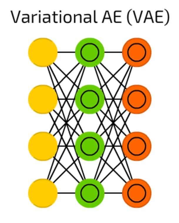
VAEs, comparing to AE, compress probabilities instead of features.
Despite that simple change, when AEs answer the question “how can we generalise data?”, VAEs answer the question “how strong is a connection between two events? should we distribute error between the two events or they are completely independent?”.
A little bit more in-depth explanation (with some code) is accessible here.
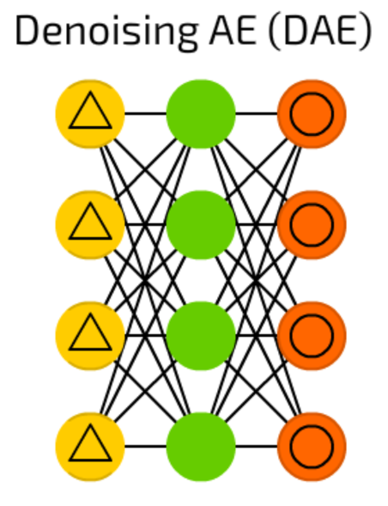
While AEs are cool, they sometimes, instead of finding the most robust features, just adapt to input data (it is actually an example of overfitting).
DAEs add a bit of noise on the input cells — vary the data by random bit, randomly switch bits in input, etc. By doing that, one forces DAE to reconstruct output from a bit noisy input, making it more general and forcing to pick more common features.
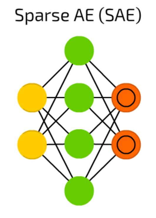
SAE is yet another autoencoder type that in some cases can reveal some hidden grouping patters in data. Structure is the same as in AE but hidden cell count is bigger than input / output layer cell count.
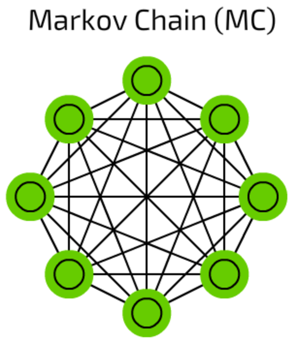
Markov Chains are pretty old concept of graphs where each edge has a probability. In old times they were used to construct texts like “after word hello we might have word dear with 0.0053% probability and word you with 0.03551% probability” (your T9, by the way, uses MCs to predict your input).
This MCs are not neural networks in a classic way, MCs can be used for classification based on probabilities (like Bayesian filters), for clustering (of some sort), and as a finite state machine.
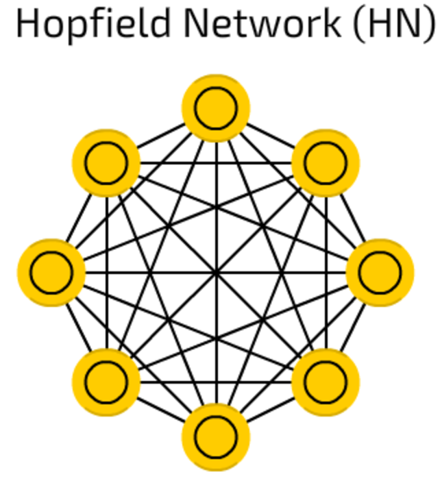
Hopfield networks are trained on a limited set of samples so they respond to a known sample with the same sample.
Each cell serves as input cell before training, as hidden cell during training and as output cell when used.
As HNs try to reconstruct the trained sample, they can be used for denoising and restoring inputs. Given a half of learned picture or sequence, they will return full sample.
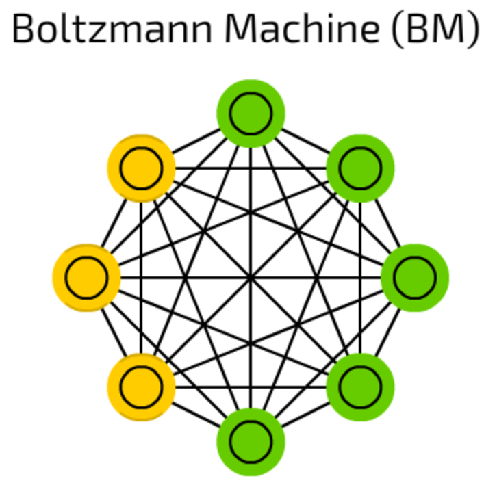
Boltzmann machines are very similar to HNs where some cells are marked as input and remain hidden. Input cells become output as soon as each hidden cell update their state (during training, BMs / HNs update cells one by one, and not in parallel).
This is the first network topology that was succesfully tained using Simulated annealing approach.
Multiple stacked Boltzmann Machines can for a so-called Deep belief network (see below), that is used for feature detection and extraction.
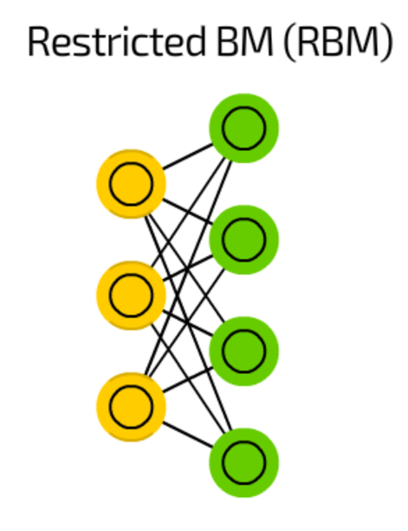
RBMs resemble, in the structure, BMs but, due to being restricted, allow to be trained using backpropagation just as FFs (with the only difference that before backpropagation pass data is passed back to input layer once).
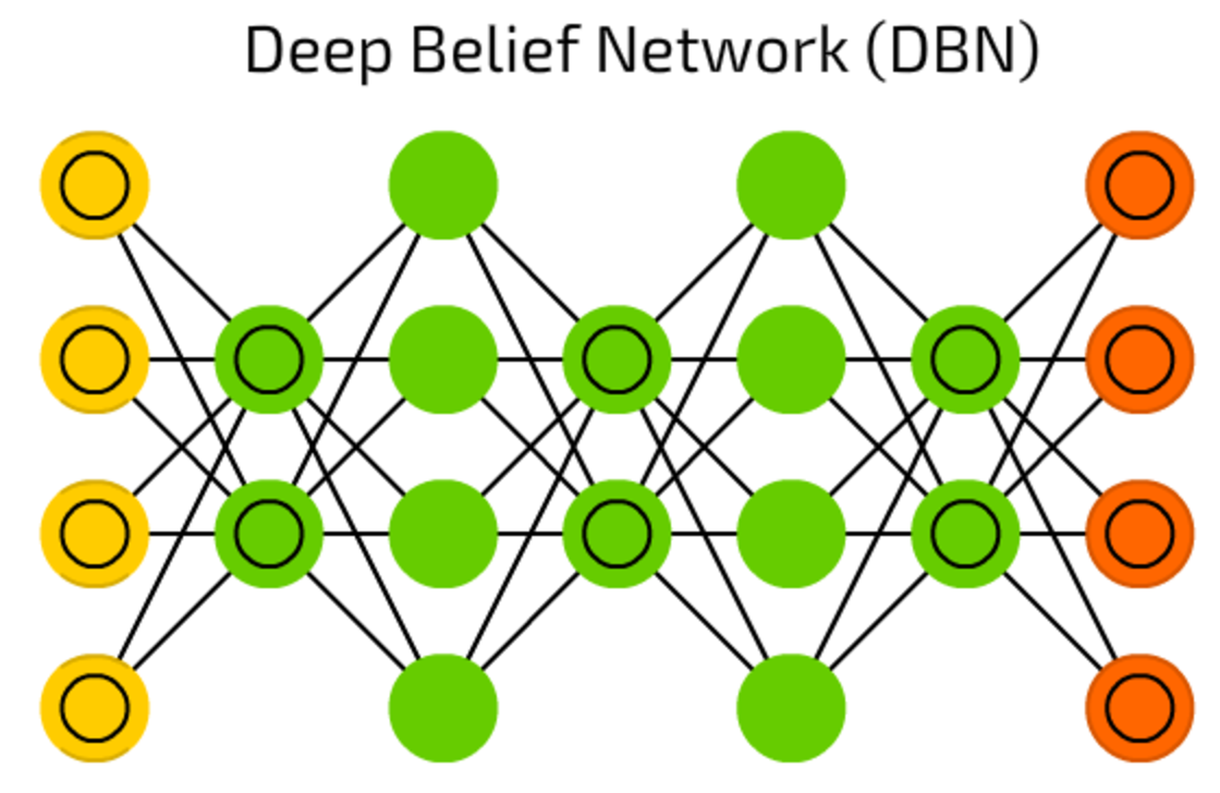
DBNs, mentioned above, are actually a stack of Boltzmann Machines (surrounded by VAEs). They can be chained together (when one NN trains another) and can be used to generate data by already learned pattern.
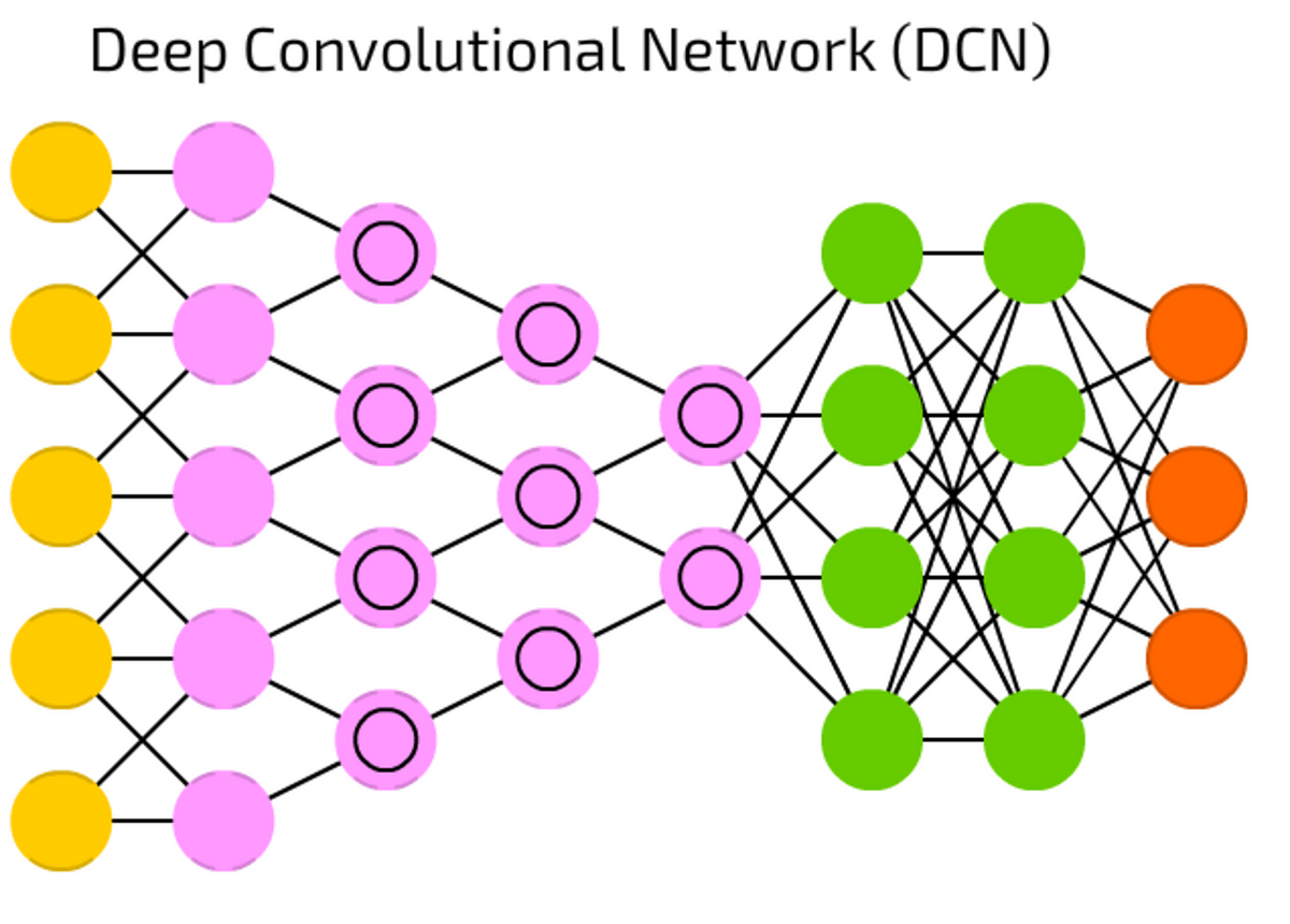
DCN nowadays are stars of artificial neural networks. They feature convolution cells (or pooling layers) and kernels, each serving a different purpose.
Convolution kernels actually process input data, and pooling layers simplify it (mostly using non-linear functions, like max), reducing unnecessary features.
Typically used for image recognition, they operate on small subset of image (something about 20x20 pixels). The input window is sliding along the image, pixel by pixel. The data is passed to convolution layers, that form a funnel (compressing detected features). From the terms of image recognition, first layer detects gradients, second lines, third shapes, and so on to the scale of particular objects. DFFs are commonly attached to the final convolutional layer for further data processing.
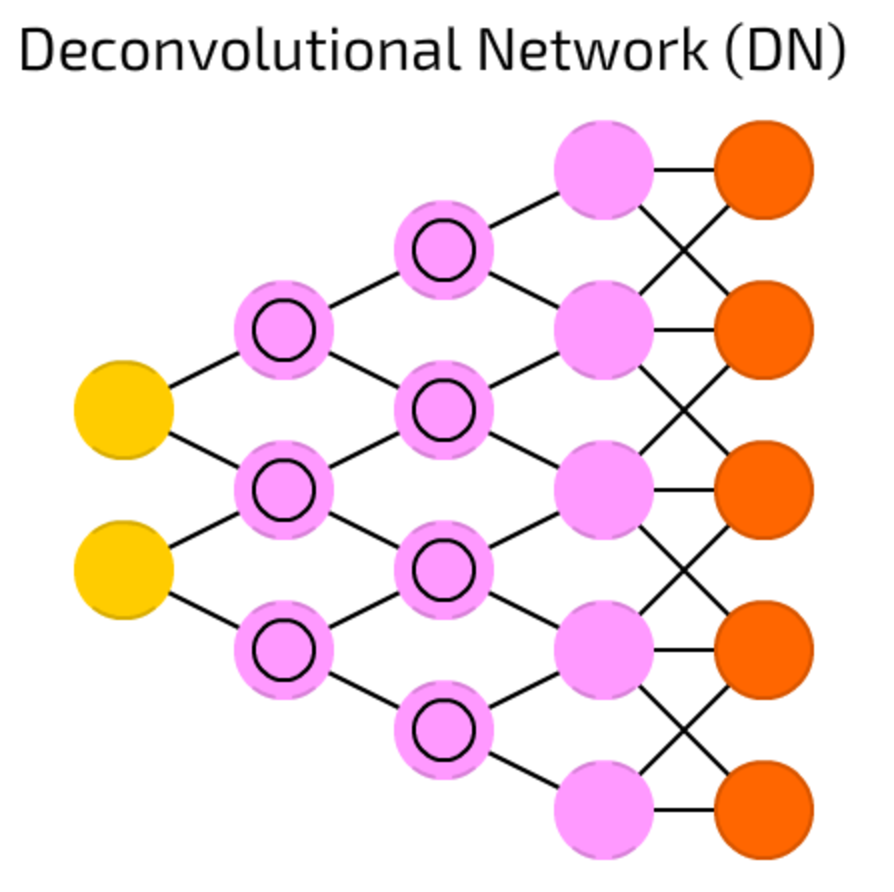
DNs are DCNs reversed. DN takes cat image, and produces vector like { dog: 0, lizard: 0, horse: 0, cat: 1 }. DCN can take this vector and draw a cat image from that. I tried to find a solid demo, but the best demo is on youtube.
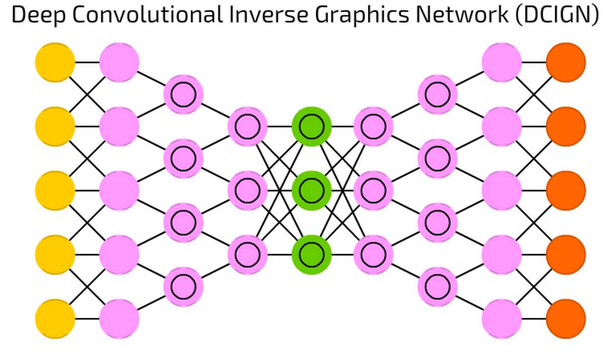
DCIGN (oh my god, this is long) looks like DCN and DN glued together, but it is not quire correct.
Actually, it is an autoencoder. DCN and DN do not act as separate networks, instead, they are spacers for input and output of the network. Mostly used for image processing, these networks can process images that they have not been trained with previously. These nets, due to their abstraction levels, can remove certain objects from image, re-paint it, or replace horses with zebras like the famous CycleGAN did.
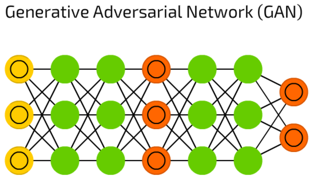
GAN represents a huge family of double networks, that are composed from generator and discriminator. They constantly try to fool each other — generator tries to generate some data, and discriminator, receiving sample data, tries to tell generated data from samples. Constantly evolving, this type of neural networks can generate real-life images, in case you are able to maintain the training balance between these two networks.
pix2pix is an excellent example of such approach.
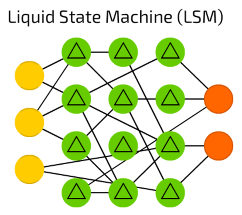
LSM is sparse (not fully connected) neural network where activation functions are replaced by threshold levels. Cell accumulates values from sequential samples, and emits output only when the threshold is reached, setting internal counter again to zero.
Such idea is taken from human brain, and these networks are widely used in computer vision and speech recognition systems, but without major breakthroughs.
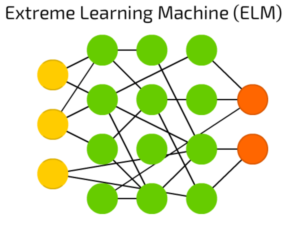
ELM is an attempt to reduce complexity behind FF networks by creating sparse hidden layers with random connections. They require less computational power, but the actual efficiency heavily depends on the task and data.
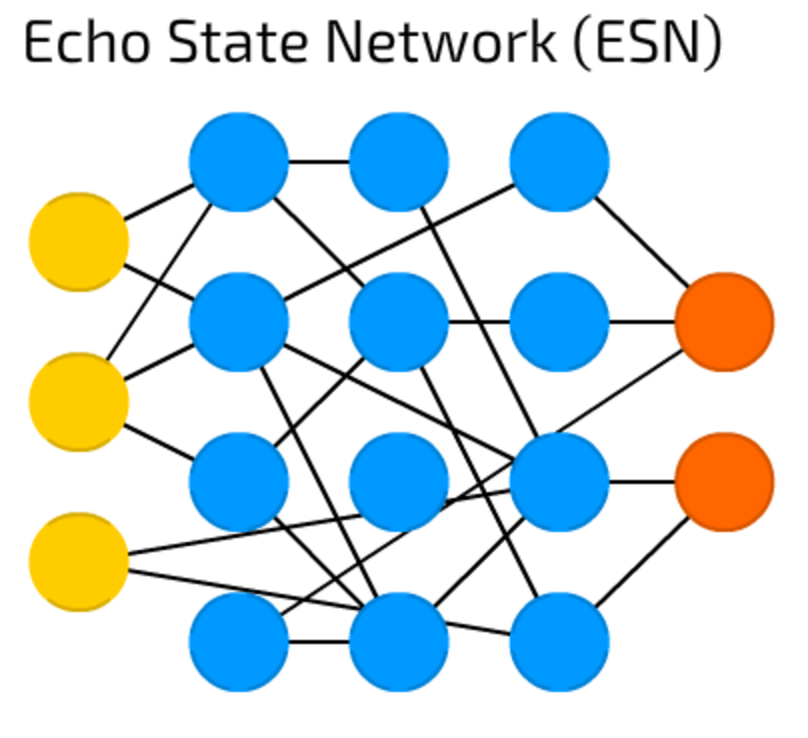
ESN is a subtype of recurrent networks with a special training approach. The data is passed to input, then the output if being monitored for multiple iterations (allowing the recurrent features to kick in). Only weights between hidden cells are updated after that.
Personally, I know no real application of that type apart of multiple theoretical benchmarks. Feel free to add yours ).
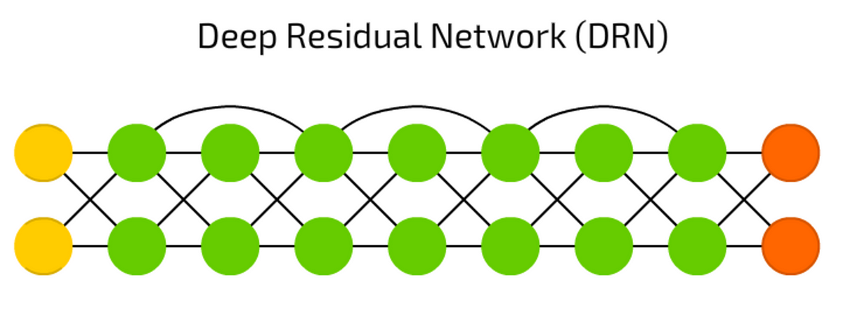
DRN is a deep network where some part of input data is passed to next layers. This feature allows them to be really deep (up to 300 layers), but actually they are kind of RNN without explicit delay.
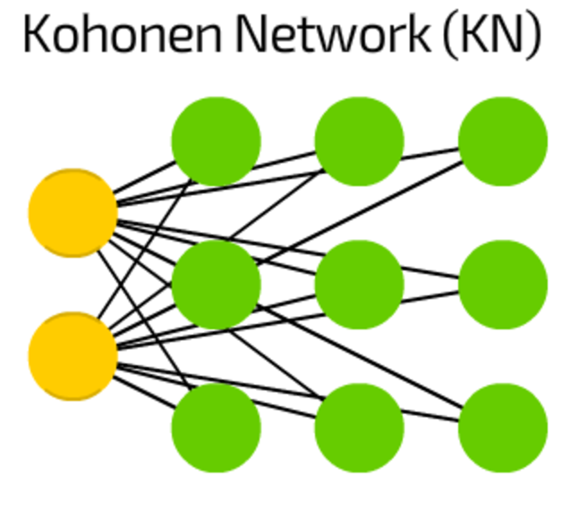
KN introduces the “distance to cell” feature. Mostly used for classification, this type of network tries to adjust their cells for maximal reaction to particular input. When some cell is updated, it’s closest neighbours are updated aswell.
Like SVMs these networks are not always considered to be a “real” neural networks.
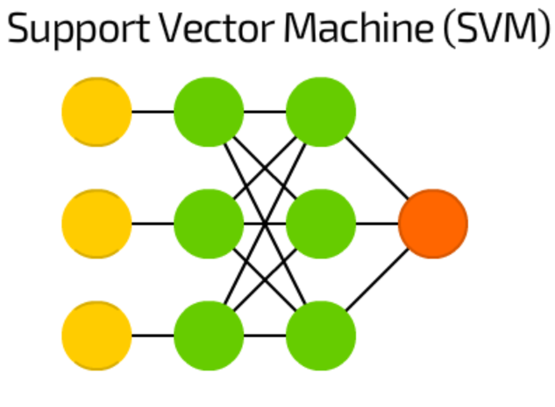
SVM is used for binary classification tasks. No matter how many dimensions — or inputs — the net may process, the answer is always “yes” or “no”.
SVMs are not always considered to be a neural network.
Huh, the last one!
Neural networks are kinda black-boxes — we can train them, get results, enhance them but the actual decision path is mostly hidden from us.
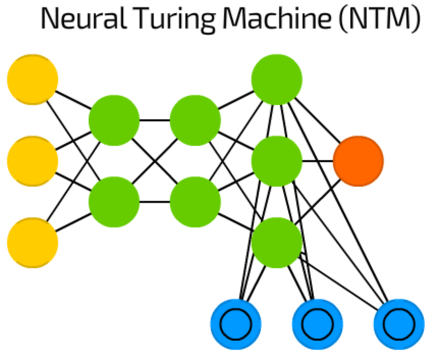
The NTM is an attempt to fix it — is it a FF with memory cells extracted. Some authors also say that it is an abstraction over LSTM.
The memory is addressed by its contents, and the network can read from and write to the memory depending on current state, representing a Turing-complete neural network.
原文地址: https://towardsdatascience.com/the-mostly-complete-chart-of-neural-networks-explained-3fb6f2367464


 6962
6962

 被折叠的 条评论
为什么被折叠?


