


This article covers the second Hinton’s capsule network paper Matrix capsules with EM Routing, both authored by Geoffrey E Hinton, Sara Sabour and Nicholas Frosst. We will first cover the matrix capsules and apply EM (Expectation Maximization) routing to classify images with different viewpoints. For those want to understand the detail implementation, the second half of the article covers an implementation on the matrix Capsule and EM routing using TensorFlow.
CNN challenges
In our previous capsule article, we cover the challenges of CNN in exploring spatial relationship and discuss how capsule networks may address those short-comings. Let’s recap some important challenges of CNN in classifying the same class of images but in different viewpoints. For example, classify a face correctly even with different orientations.
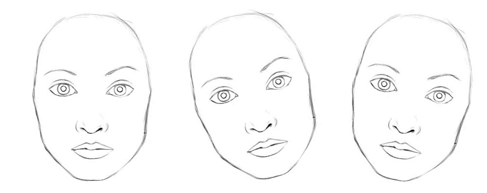
Conceptually, the CNN trains neurons to handle different feature orientations (0°, 20°, -20° ) with a top level face detection neuron.
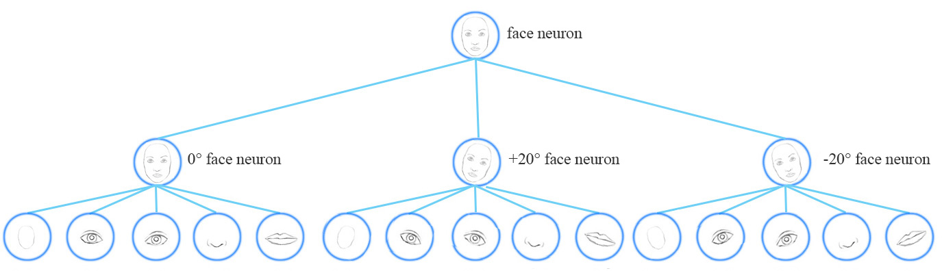
To solve the problem, we add more convolution layers and features maps. Nevertheless this approach tends to memorize the dataset rather than generalize a solution. It requires a large volume of training data to cover different variants and to avoid overfitting. MNist dataset contains 55,000 training data. i.e. 5,500 samples per digits. However, it is unlikely that children need so many samples to learn numbers. Our existing deep learning models including CNN are inefficient in utilizing datapoints.
Adversaires
CNN is also vulnerable to adversaires by simply move, rotate or resize individual features.
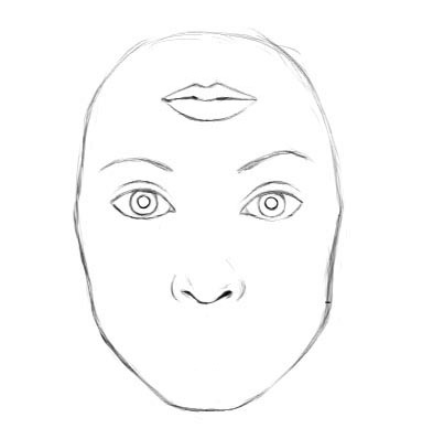
We can add tiny un-noticeable changes to an image to fool a deep network easily. The image on the left below is correctly classified by a CNN network as a panda. By selectively adding small changes from the middle picture to the panda picture, the CNN suddenly mis-classifies the resulting image in the right as a gibbon.
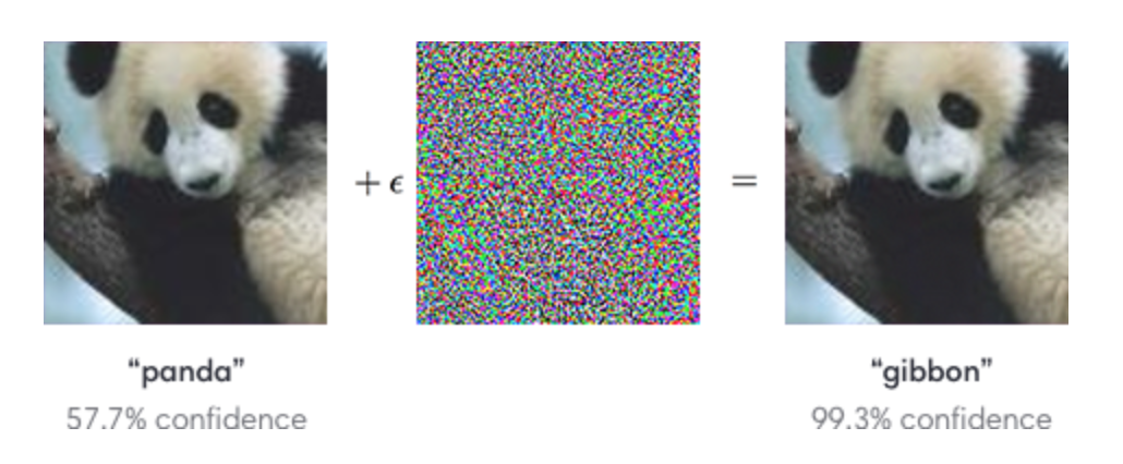
(image source OpenAi)
Capsule
A capsule captures the likeliness of a feature and its variant. So the capsule does not only detect a feature but it is trained to learn and detect the variants.
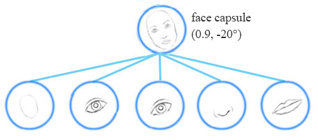
For example, the same network layer can detect a face rotated clockwise.
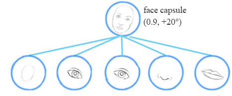
Equivariance is the detection of objects that can transform to each other. Intuitively, the capsule network detects the face is rotated right 20° (an equivariance) rather than realizes the face matched a variant that is rotated 20°. By forcing the model to learn the feature variant in a capsule, we may extrapolate possible variants more effectively with less training data. In CNN, the final label is viewpoint invariant. i.e. the top neuron detects a face but losses the information in the angle of rotation. For equivariance, the variant information like the angle of rotation is kept inside the capsule. Maintaining such spatial orientation helps us to avoid adversaires.
Matrix capsule
A matrix capsule captures the activation (likeliness) similar to that of a neuron, but also captures a 4x4 pose matrix. In computer graphics, a pose matrix defines the translation and the rotation of an object which is equivalent to the change of the viewpoint of an object.

(Source from the Matrix capsules with EM routing paper)
For example, the second row images below represent the same object above them with differen viewpoints. In matrix capsule, we train the model to capture the pose information (orientation, azimuths etc…). Of course, just like other deep learning methods, this is our intention and it is never guaranteed.
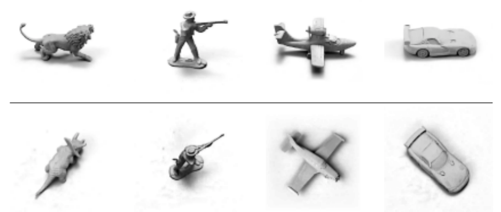
(Source from the Matrix capsules with EM routing paper)
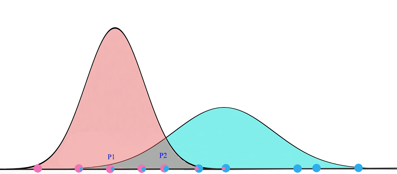
The objective of the EM (Expectation Maximization) routing is to group capsules to form a part-whole relationship using a clustering technique (EM). In machine learning, we use EM clustering to cluster datapoints into Gaussian distributions. For example, we cluster the datapoints below into two clusters modeled by two gaussian distributions G1=N(μ1,σ21)G1=N(μ1,σ12) and G2=N(μ2,σ22)G2=N(μ2,σ22). Then we represent the datapoints by the corresponding Gaussian distribution.
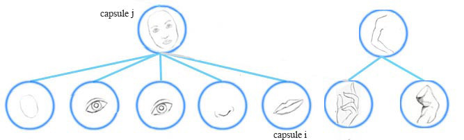
In the face detection example, each of the mouth, eyes and nose detection capsules in the lower layer makes predictions (votes) on the pose matrices of its possible parent capsules. Each vote is a predicted value for a parent capsule’s pose matrix, and it is computed by multiplying its own pose matrix MM with a transformation matrix WW that we learn from the training data.
We apply the EM routing to group capsules into a parent capsule in runtime:
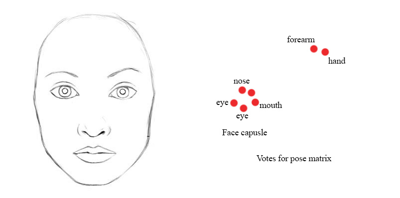
i.e., if the nose, mouth and eyes capsules all vote a similar pose matrix value, we cluster them together to form a parent capsule: the face capsule.
A higher level feature (a face) is detected by looking for agreement between votes from the capsules one layer below. We use EM routing to cluster capsules that have close proximity of the corresponding votes.
Gaussian mixture model & Expectation Maximization (EM)
We will take a short break to understand EM. A Gaussian mixture model clusters datapoints into a mixture of Gaussian distributions described by a mean μμ and a standard deviation σσ. Below, we cluster datapoints into the yellow and red cluster which each is described by a μμ and a σσ.
(Image source Wikipedia)
For a Gaussian mixture model with two clusters, we start with a random initialization of clusters G1=(μ1,σ21)G1=(μ1,σ12)and G2=(μ2,σ22)G2=(μ2,σ22). Expectation Maximization (EM) algorithm tries to fit the training datapoints into G1G1 and G2G2and then re-compute μμ and σσ for G1G1 and G2G2 based on Gaussian distribution. The iteration continues until the solution converged such that the probability of seeing all datapoints is maximized with the final G1G1 and G2G2distribution.
The probability of xx given (belong to) the cluster G1G1 is:
At each iteration, we start with 2 Gaussian distributions which we later re-calculate its μμ and σσ based on the datapoints.
Eventually, we will converge to two Gaussian distributions that maximize the likelihood of the observed datapoints.
Using EM for Routing-By-Agreement
Now, let’s get into more details. A higher level feature (a face) is detected by looking for agreement between votes from the capsules one layer below. A vote vijvij for the parent capsule jj from capsule ii is computed by multipling the pose matrix MiMi of capsule ii with a viewpoint invariant transformation WijWij.
The probability that a capsule ii is grouped into capsule jj as a part-whole relationship is based on the proximity of the vote vijvij to other votes (vo1j…vokj)(vo1j…vokj) from other capsules. WijWij is learned discriminatively through a cost function and the backpropagation. It learns not only what a face is composed of, and it also makes sure the pose information of the parent capsule matched with its sub-components after some transformation.
Here is the visualization of routing-by-agreement with the matrix capsules. We group capsules with similar votes (TiTij≈ThThjTiTij≈ThThj) after transform the pose TiTi and TjTj with a viewpoint invariant transformation. (TijTij aka WijWijand ThjThj)
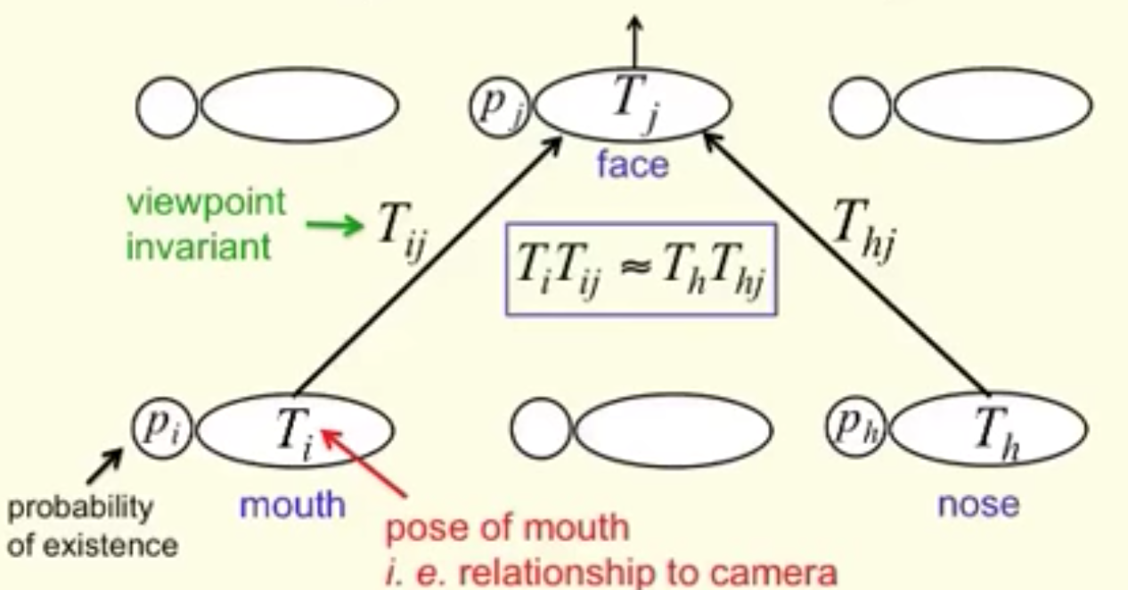
(Source Geoffrey Hinton)
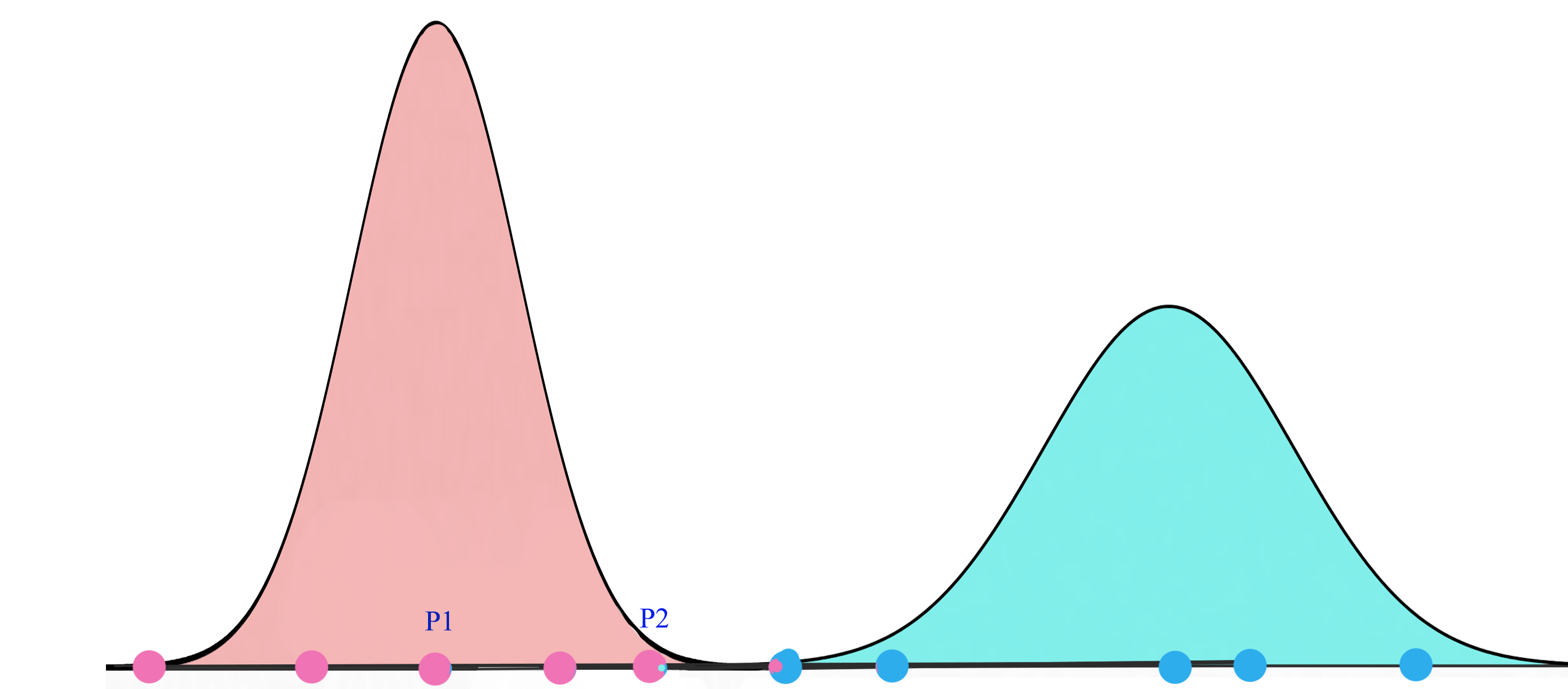
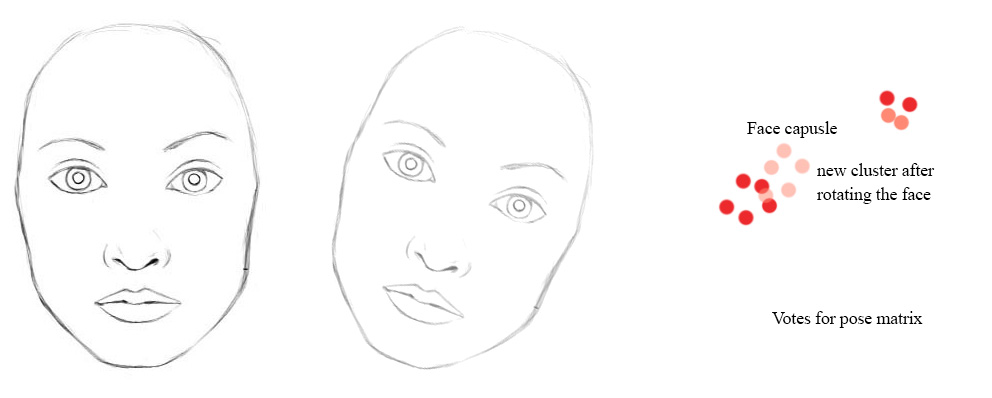
Even the viewpoint may change, the pose matrices and the votes change in a co-ordinate way. In our example, the locations of the votes may change from the red dots to the pink dots below when the face is rotated. Nevertheless, EM routing is based on proximity and therefore EM routing can still cluster the same children capsules together. Hence, the transformation matrices are the same for any viewpoints of the objects: viewpoint invariant. We just need one set of the transformation matrices and one parent capsule for different object orientations.
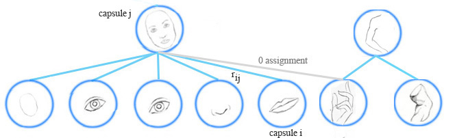
Capsule assignment
EM routing clusters capsules to form a higher level capsule in runtime. It also calculates the assignment probabilities rijrij to quantify the runtime connection between a capsule and its parents. For example, the hand capsule does not belong to the face capsule, the assignment probability between them is zero. rijrij is also impacted by the activation of a capsule. If the mouth in the image is obstructed, the mouth capsule will have zero activation. The calculated rijrij will also be zero.
Calculate capsule activation and pose matrix
The output of a capsule is computed differently than a deep network neuron. In EM clustering, we represent datapoints by a Gaussian distribution. In EM routing, we model the pose matrix of the parent capsule with a Gaussian also. The pose matrix is a 4×44×4 matrix, i.e. 16 components. We model the pose matrix with a Gaussian having 16 μμ and 16 σσ and each μμ represents a pose matrix’s component.
Let vijvij be the vote from capsule ii for the parent capsule jj, and vhijvijh be its hh-th component. We apply the probability density function of a Gaussian
to compute the probability of vhijvijh belonging to the capsule jj’s Gaussian model:
Let’s take the natural loglog:
Let’s estimate the cost to activate a capsule. The lower the cost, the more likely a capsule will be activated. If cost is high, the votes do not match the parent Gaussian distribution and therefore a low chance to be activated.
Let costijcostij be the cost to activate the parent capsule jj by the capsule ii. It is the negative of the log likelihood:
Since capsules are not equally linked with capsule jj, we pro-rated the cost with the runtime assignment probabilities rijrij. The cost from all lower layer capsules is:
To determine whether the capsule jj will be activated, we use the following equation:
In the original paper, “−bj−bj” is explained as the cost of describing the mean and variance of capsule jj. In another word, if the benefit bjbj of representing datapoints by the parent capsule jj outranks the cost caused by the discrepancy in their votes, we activate the output capsules. We do not compute bjbj analytically. Instead, we approximate it through training using the backpropagation and a cost function.
rijrij, μμ, σσ and ajaj are computed iteratively using EM routing discussed in the next section. λ in the equation above is the inverse temperature parameter 1temperature1temperature. As rijrij is getting better, we drop the temperature (larger λ) which increase the steepness in the s-curve in sigmoid(z)sigmoid(z). It helps us to fine tune rijrij better with higher sensitivity to vote discrepancy in these region. In our implementation, λ is first initialized to 1 at the beginning of the iterations and then increment by 1 after each routing iteration. The paper does not specific the details and we would suggest experimenting different schemes in your implementation.
EM Routing
The pose matrix and the activation of the output capsules are computed iteratively using the EM routing. The EM method fits datapoints into a a mixture of Gaussian models with alternative calls between an E-step and an M-step. The E-step determines the assignment probability rijrij of each datapoint to a parent capsule. The M-step re-calculate the Gaussian models’ values based on rijrij. We repeat the iteration 3 times. The last ajaj will be the parent capsule’s output. The 16 μμ from the last Gaussian model will be reshaped to form the 4×44×4 pose matrix of the parent capsule.
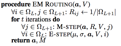
(Source from the Matrix capsules with EM routing paper)
aa and VV above is the activation and the votes from the children capsules. We initialize the assignment probability rijrij to be uniformly distributed. i.e. we start with the children capsules equally related with any parents. We call M-step to compute an updated Gaussian model (μμ, σσ) and the parent activation ajaj from aa, VVand current rijrij. Then we call E-step to recompute the assignment probabilities rijrij based on the new Gaussian model and the new ajaj.
The details of M-step:
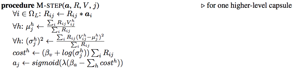
In M-step, we calculate μμ and σσ based on the activation aiai from the children capsules, the current rijrij and votes VV. M-step also re-calcule the cost and the activation ajaj for the parent capsules. βνβν and βαβα is trained discriminatively. λ is an inverse temperature parameter increased by 1 after each routing iteration in our code implementation.
The details of E-step:
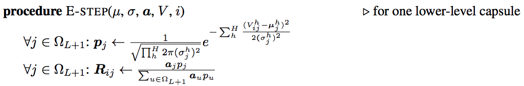
In E-step, we re-calculate the assignment probability rijrij based on the new μμ, σσ and ajaj. The assignment is increased if the vote is closer to the μμ of the updated Gaussian model.
We use the ajaj from the last m-step call in the iterations as the activation of the output capsule jj and we shape the 16 μμ to form the 4x4 pose matrix.
The role of backpropagation & EM routing
In CNN, we use the formula below to calculate the activation of a neuron.
However, the output of a capsule including the activation and the pose matrix is calculated by the EM routing. We use EM-routing to compute the parent capsule’s output from the transformation matrix WW and the children capsules’ activations and pose matrices. Nevertheless, by no mistake, the matrix capsules still heavily depend on the backpropagation in training the transformation matrix WijWij and the parameters βνβν and βαβα.
In EM routing, we compute the assignment probability rijrij to quantify the connection between the children capsules and the parent capsules. This value is important but short lived. We re-initialize it to be uniformly distributed for every datapoint before the EM routing calculation. In any situration, training or testing, we use EM routing to compute capsules’ outputs.
Loss function (using Spread loss)
Matrix capsules requires a loss function to train WW, βνβν and βαβα. We pick spread loss as the main loss function for the backpropagation. The loss from the class ii (other than the true label tt) is defined as
which atat is the activation of the target class (true label) and aiai is the activation for class ii.
The total cost is:
If the margin between the true label and the wrong class is smaller than mm, we penalize it by the square of m−(at−ai)m−(at−ai). mm is initially start as 0.2 and linearly increased by 0.1 after each epoch training. mm will stop growing after reaching the maximum 0.9. Starting at a lower margin helps the training to avoid too many dead capsules during the early phase.
Other implementations add regularization loss and reconstruction loss to the loss function. Since those are not specific to the matrix capsule, we will simply mention here without further elaboration.
Capsule Network
The Capsule Network (CapsNet) in the first paper uses a fully connected network. This solution is hard to scale for larger images. In the next few sections, the matrix capsules use some of the convolution techniques in CNN to explore spatial features so it can scale better.
smallNORB
The research paper uses the smallNORB dataset. It has 5 toy classes: airplanes, cars, trucks, humans and animals. Every individual sample is pictured at 18 different azimuths (0-340), 9 elevations and 6 lighting conditions. This dataset is particular picked by the paper so it can study the classification of images with different viewpoints.
(Picture from the Matrix capsules with EM routing paper)
Architect
However, many code implementations start with the MNist dataset because the image size is smaller. So for our demonstration, we also pick the MNist dataset. This is the network design:
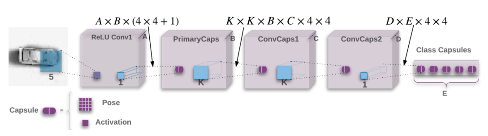
(Picture from the Matrix capsules with EM routing paper).
ReLU Conv1 is a regular convolution (CNN) layer using a 5x5 filter with stride 2 outputting 32 (A=32A=32) channels (feature maps) using the ReLU activation.
In PrimaryCaps, we apply a 1x1 convolution filter to transform each of the 32 channels into 32 (B=32B=32) primary capsules. Each capsule contains a 4x4 pose matrix and an activation value. We use the regular convolution layer to implement the PrimaryCaps. We group 4×4+14×4+1 neurons to generate 1 capsule.
PrimaryCaps is followed by a convolution capsule layer ConvCaps1 using a 3x3 filters (K=3K=3) with stride 2. ConvCaps1 takes capsules as input and output capsules. ConvCaps1 is similar to a regular convolution layer except it uses EM routing to compute the capsule output.
The capsule output of ConvCaps1 is then feed into ConvCaps2. ConvCaps2 is another convolution capsule layer but with stride 1.
The output capsules of ConvCaps2 are connected to the Class Capsules using a 1x1 filter and it outputs one capsule per class. (In MNist, we have 10 classes E=10E=10)
We use EM routing to compute the pose matrices and the output activations for ConvCaps1, ConvCaps2 and Class Capsules. In CNN, we slide the same filter over the spatial dimension in calculating the same feature map. We want to detect the same feature regardless of the location. Similarly, in EM routing, we share the same transformation matrix WijWij across spatial dimension to calculate the votes.
For example, from ConvCaps1 to ConvCaps2, we have
- a 3x3 filter,
- 32 input and output capsules, and
- a 4x4 pose matrix.
Since we share the transformation matrix, we just need 3x3x32x32x4x4 parameters for WW.
Here is the summary of each layer and the shape of their outputs:
| Layer Name | Apply | Output shape |
|---|---|---|
| MNist image | 28, 28, 1 | |
| ReLU Conv1 | Regular Convolution (CNN) layer using 5x5 kernels with 32 output channels, stride 2 and padding | 14, 14, 32 |
| PrimaryCaps | Modified convolution layer with 1x1 kernels, strides 1 with padding and outputing 32 capsules. Requiring 32x32x(4x4+1) parameters. | pose (14, 14, 32, 4, 4), activations (14, 14, 32) |
| ConvCaps1 | Capsule convolution with 3x3 kernels, strides 2 and no padding. Requiring 3x3x32x32x4x4 parameters. | poses (6, 6, 32, 4, 4), activations (6, 6, 32) |
| ConvCaps2 | Capsule convolution with 3x3 kernels, strides 1 and no padding | poses (4, 4, 32, 4, 4), activations (4, 4, 32) |
| Class Capsules | Capsule with 1x1 kernel. Requiring 32x10x4x4 parameters. | poses (10, 4, 4), activations (10) |
For the rest of the article, we will cover a detail implementation using Tensor. Here is the code in building our layers:
def capsules_net(inputs, num_classes, iterations, batch_size, name='capsule_em'):
    """Define the Capsule Network model
    """

    with tf.variable_scope(name) as scope:
        # ReLU Conv1
        # Images shape (24, 28, 28, 1) -> conv 5x5 filters, 32 output channels, strides 2 with padding, ReLU
        # nets -> (?, 14, 14, 32)
        nets = conv2d(
            inputs,
            kernel=5, out_channels=32, stride=2, padding='SAME',
            activation_fn=tf.nn.relu, name='relu_conv1'
        )

        # PrimaryCaps
        # (?, 14, 14, 32) -> capsule 1x1 filter, 32 output capsule, strides 1 without padding
        # nets -> (poses (?, 14, 14, 32, 4, 4), activations (?, 14, 14, 32))
        nets = primary_caps(
            nets,
            kernel_size=1, out_capsules=32, stride=1, padding='VALID',
            pose_shape=[4, 4], name='primary_caps'
        )

        # ConvCaps1
        # (poses, activations) -> conv capsule, 3x3 kernels, strides 2, no padding
        # nets -> (poses (24, 6, 6, 32, 4, 4), activations (24, 6, 6, 32))
        nets = conv_capsule(
            nets, shape=[3, 3, 32, 32], strides=[1, 2, 2, 1], iterations=iterations,
            batch_size=batch_size, name='conv_caps1'
        )

        # ConvCaps2
        # (poses, activations) -> conv capsule, 3x3 kernels, strides 1, no padding
        # nets -> (poses (24, 4, 4, 32, 4, 4), activations (24, 4, 4, 32))
        nets = conv_capsule(
            nets, shape=[3, 3, 32, 32], strides=[1, 1, 1, 1], iterations=iterations,
            batch_size=batch_size, name='conv_caps2'
        )

        # Class capsules
        # (poses, activations) -> 1x1 convolution, 10 output capsules
        # nets -> (poses (24, 10, 4, 4), activations (24, 10))
        nets = class_capsules(nets, num_classes, iterations=iterations,
                              batch_size=batch_size, name='class_capsules')

        # poses (24, 10, 4, 4), activations (24, 10)
        poses, activations = nets

    return poses, activations
ReLU Conv1
ReLU Conv1 is a simple CNN layer. We use the TensorFlow slim API slim.conv2d to create a CNN layer using a 3x3 kernel with stride 2 and ReLU. (We use the slim API so the code is more condense and easier to read.)
def conv2d(inputs, kernel, out_channels, stride, padding, name, is_train=True, activation_fn=None):
  with slim.arg_scope([slim.conv2d], trainable=is_train):
    with tf.variable_scope(name) as scope:
      output = slim.conv2d(inputs,
                           num_outputs=out_channels,
                           kernel_size=[kernel, kernel], stride=stride, padding=padding,
                           scope=scope, activation_fn=activation_fn)
      tf.logging.info(f"{name} output shape: {output.get_shape()}")

  return output
PrimaryCaps
PrimaryCaps is not much difference from a CNN layer: instead of generating 1 scalar value, we generate 32 capsules with 4 x 4 scalar values for the pose matrices and 1 scalar for the activation:
def primary_caps(inputs, kernel_size, out_capsules, stride, padding, pose_shape, name):
    """This constructs a primary capsule layer using regular convolution layer.

    :param inputs: shape (N, H, W, C) (?, 14, 14, 32)
    :param kernel_size: Apply a filter of [kernel, kernel] [5x5]
    :param out_capsules: # of output capsule (32)
    :param stride: 1, 2, or ... (1)
    :param padding: padding: SAME or VALID.
    :param pose_shape: (4, 4)
    :param name: scope name

    :return: (poses, activations), (poses (?, 14, 14, 32, 4, 4), activations (?, 14, 14, 32))
    """

    with tf.variable_scope(name) as scope:
        # Generate the poses matrics for the 32 output capsules
        poses = conv2d(
            inputs,
            kernel_size, out_capsules * pose_shape[0] * pose_shape[1], stride, padding=padding,
            name='pose_stacked'
        )

        input_shape = inputs.get_shape()

        # Reshape 16 scalar values into a 4x4 matrix
        poses = tf.reshape(
            poses, shape=[-1, input_shape[-3], input_shape[-2], out_capsules, pose_shape[0], pose_shape[1]],
            name='poses'
        )

        # Generate the activation for the 32 output capsules
        activations = conv2d(
            inputs,
            kernel_size,
            out_capsules,
            stride,
            padding=padding,
            activation_fn=tf.sigmoid,
            name='activation'
        )

        tf.summary.histogram(
            'activations', activations
        )

    # poses (?, 14, 14, 32, 4, 4), activations (?, 14, 14, 32)
    return poses, activations
ConvCaps1, ConvCaps2
ConvCaps1 and ConvCaps are both convolution capsule with stride 2 and 1 respectively. In the comment of the following code, we trace the tensor shape for the ConvCaps1 layer.
The code involves 3 major steps:
- Use kernel_tile to tile (convolute) the pose matrices and the activation to be used later in voting and EM routing.
- Compute votes: call mat_transform to generate the votes from the children “tiled” pose matrices and the transformation matrices.
- EM-routing: call matrix_capsules_em_routing to compute the output capsules (pose and activation) of the parent capsule.
def conv_capsule(inputs, shape, strides, iterations, batch_size, name):
  """This constructs a convolution capsule layer from a primary or convolution capsule layer.
      i: input capsules (32)
      o: output capsules (32)
      batch size: 24
      spatial dimension: 14x14
      kernel: 3x3
  :param inputs: a primary or convolution capsule layer with poses and activations
         pose: (24, 14, 14, 32, 4, 4)
         activation: (24, 14, 14, 32)
  :param shape: the shape of convolution operation kernel, [kh, kw, i, o] = (3, 3, 32, 32)
  :param strides: often [1, 2, 2, 1] (stride 2), or [1, 1, 1, 1] (stride 1).
  :param iterations: number of iterations in EM routing. 3
  :param name: name.

  :return: (poses, activations).

  """
  inputs_poses, inputs_activations = inputs

  with tf.variable_scope(name) as scope:

      stride = strides[1] # 2
      i_size = shape[-2] # 32
      o_size = shape[-1] # 32
      pose_size = inputs_poses.get_shape()[-1]  # 4

      # Tile the input capusles' pose matrices to the spatial dimension of the output capsules
      # Such that we can later multiple with the transformation matrices to generate the votes.
      inputs_poses = kernel_tile(inputs_poses, 3, stride)  # (?, 14, 14, 32, 4, 4) -> (?, 6, 6, 3x3=9, 32x16=512)

      # Tile the activations needed for the EM routing
      inputs_activations = kernel_tile(inputs_activations, 3, stride)  # (?, 14, 14, 32) -> (?, 6, 6, 9, 32)
      spatial_size = int(inputs_activations.get_shape()[1]) # 6

      # Reshape it for later operations
      inputs_poses = tf.reshape(inputs_poses, shape=[-1, 3 * 3 * i_size, 16])  # (?, 9x32=288, 16)
      inputs_activations = tf.reshape(inputs_activations, shape=[-1, spatial_size, spatial_size, 3 * 3 * i_size]) # (?, 6, 6, 9x32=288)

      with tf.variable_scope('votes') as scope:

          # Generate the votes by multiply it with the transformation matrices
          votes = mat_transform(inputs_poses, o_size, size=batch_size*spatial_size*spatial_size)  # (864, 288, 32, 16)

          # Reshape the vote for EM routing
          votes_shape = votes.get_shape()
          votes = tf.reshape(votes, shape=[batch_size, spatial_size, spatial_size, votes_shape[-3], votes_shape[-2], votes_shape[-1]]) # (24, 6, 6, 288, 32, 16)
          tf.logging.info(f"{name} votes shape: {votes.get_shape()}")

      with tf.variable_scope('routing') as scope:

          # beta_v and beta_a one for each output capsule: (1, 1, 1, 32)
          beta_v = tf.get_variable(
              name='beta_v', shape=[1, 1, 1, o_size], dtype=tf.float32,
              initializer=initializers.xavier_initializer()
          )
          beta_a = tf.get_variable(
              name='beta_a', shape=[1, 1, 1, o_size], dtype=tf.float32,
              initializer=initializers.xavier_initializer()
          )

          # Use EM routing to compute the pose and activation
          # votes (24, 6, 6, 3x3x32=288, 32, 16), inputs_activations (?, 6, 6, 288)
          # poses (24, 6, 6, 32, 16), activation (24, 6, 6, 32)
          poses, activations = matrix_capsules_em_routing(
              votes, inputs_activations, beta_v, beta_a, iterations, name='em_routing'
          )

          # Reshape it back to 4x4 pose matrix
          poses_shape = poses.get_shape()
          # (24, 6, 6, 32, 4, 4)
          poses = tf.reshape(
              poses, [
                  poses_shape[0], poses_shape[1], poses_shape[2], poses_shape[3], pose_size, pose_size
              ]
          )

      tf.logging.info(f"{name} pose shape: {poses.get_shape()}")
      tf.logging.info(f"{name} activations shape: {activations.get_shape()}")

      return poses, activations
kernel_tile use tiling and convolution to prepare the input pose matrices and the activations to the correct spatial dimension for voting and EM-routing. (The code is pretty hard to understand so readers may simply treat it as a black box if it is too hard.)
def kernel_tile(input, kernel, stride):
    """This constructs a primary capsule layer using regular convolution layer.

    :param inputs: shape (?, 14, 14, 32, 4, 4)
    :param kernel: 3
    :param stride: 2

    :return output: (50, 5, 5, 3x3=9, 136)
    """

    # (?, 14, 14, 32x(16)=512)
    input_shape = input.get_shape()
    size = input_shape[4]*input_shape[5] if len(input_shape)>5 else 1
    input = tf.reshape(input, shape=[-1, input_shape[1], input_shape[2], input_shape[3]*size])


    input_shape = input.get_shape()
    tile_filter = np.zeros(shape=[kernel, kernel, input_shape[3],
                                  kernel * kernel], dtype=np.float32)
    for i in range(kernel):
        for j in range(kernel):
            tile_filter[i, j, :, i * kernel + j] = 1.0 # (3, 3, 512, 9)

    # (3, 3, 512, 9)
    tile_filter_op = tf.constant(tile_filter, dtype=tf.float32)

    # (?, 6, 6, 4608)
    output = tf.nn.depthwise_conv2d(input, tile_filter_op, strides=[
                                    1, stride, stride, 1], padding='VALID')

    output_shape = output.get_shape()
    output = tf.reshape(output, shape=[-1, output_shape[1], output_shape[2], input_shape[3], kernel * kernel])
    output = tf.transpose(output, perm=[0, 1, 2, 4, 3])

    # (?, 6, 6, 9, 512)
    return output
mat_transform extracts the transformation matrices parameters as a TensorFlow trainable variable ww. It then multiplies with the “tiled” input pose matrices to generate the votes for the parent capsules.
def mat_transform(input, output_cap_size, size):
    """Compute the vote.

    :param inputs: shape (size, 288, 16)
    :param output_cap_size: 32

    :return votes: (24, 5, 5, 3x3=9, 136)
    """

    caps_num_i = int(input.get_shape()[1]) # 288
    output = tf.reshape(input, shape=[size, caps_num_i, 1, 4, 4]) # (size, 288, 1, 4, 4)

    w = slim.variable('w', shape=[1, caps_num_i, output_cap_size, 4, 4], dtype=tf.float32,
                      initializer=tf.truncated_normal_initializer(mean=0.0, stddev=1.0)) # (1, 288, 32, 4, 4)
    w = tf.tile(w, [size, 1, 1, 1, 1])  # (24, 288, 32, 4, 4)

    output = tf.tile(output, [1, 1, output_cap_size, 1, 1]) # (size, 288, 32, 4, 4)

    votes = tf.matmul(output, w) # (24, 288, 32, 4, 4)
    votes = tf.reshape(votes, [size, caps_num_i, output_cap_size, 16]) # (size, 288, 32, 16)

    return votes
EM routing coding
Here is the code implementation for the EM routing which calling m_step and e_step alternatively. By default, we ran the iterations 3 times. The main purpose of the EM routing is to compute the pose matrices and the activations of the output capsules. In the last iteration, the m_step already complete the last calculation of those parameters. Therefore we skip the e_step in the last iteration which mainly responsible for re-calculating the routing assignment rijrij. The comments contain the tracing of the shape of tensors in ConvCaps1.
def matrix_capsules_em_routing(votes, i_activations, beta_v, beta_a, iterations, name):
  """The EM routing between input capsules (i) and output capsules (j).

  :param votes: (N, OH, OW, kh x kw x i, o, 4 x 4) = (24, 6, 6, 3x3*32=288, 32, 16)
  :param i_activation: activation from Level L (24, 6, 6, 288)
  :param beta_v: (1, 1, 1, 32)
  :param beta_a: (1, 1, 1, 32)
  :param iterations: number of iterations in EM routing, often 3.
  :param name: name.

  :return: (pose, activation) of output capsules.
  """

  votes_shape = votes.get_shape().as_list()

  with tf.variable_scope(name) as scope:

    # Match rr (routing assignment) shape, i_activations shape with votes shape for broadcasting in EM routing

    # rr: [3x3x32=288, 32, 1]
    # rr: routing matrix from each input capsule (i) to each output capsule (o)
    rr = tf.constant(
      1.0/votes_shape[-2], shape=votes_shape[-3:-1] + [1], dtype=tf.float32
    )

    # i_activations: expand_dims to (24, 6, 6, 288, 1, 1)
    i_activations = i_activations[..., tf.newaxis, tf.newaxis]

    # beta_v and beta_a: expand_dims to (1, 1, 1, 1, 32, 1]
    beta_v = beta_v[..., tf.newaxis, :, tf.newaxis]
    beta_a = beta_a[..., tf.newaxis, :, tf.newaxis]

    # inverse_temperature schedule (min, max)
    it_min = 1.0
    it_max = min(iterations, 3.0)
    for it in range(iterations):
      inverse_temperature = it_min + (it_max - it_min) * it / max(1.0, iterations - 1.0)
      o_mean, o_stdv, o_activations = m_step(
        rr, votes, i_activations, beta_v, beta_a, inverse_temperature=inverse_temperature
      )

      # We skip the e_step call in the last iteration because we only
      # need to return the a_j and the mean from the m_stp in the last iteration
      # to compute the output capsule activation and pose matrices
      if it < iterations - 1:
        rr = e_step(
          o_mean, o_stdv, o_activations, votes
        )

    # pose: (N, OH, OW, o 4 x 4) via squeeze o_mean (24, 6, 6, 32, 16)
    poses = tf.squeeze(o_mean, axis=-3)

    # activation: (N, OH, OW, o) via squeeze o_activationis [24, 6, 6, 32]
    activations = tf.squeeze(o_activations, axis=[-3, -1])

  return poses, activations
In the equation for the output capsule’s activation ajaj
λ is an inverse temperature parameter. In our implementation, we start from 1 and increment it by 1 after each routing iteration. The original paper does not specify how λ is increased and you can experiment different schemes instead. Here is our source code:
# inverse_temperature schedule (min, max)
it_min = 1.0
it_max = min(iterations, 3.0)
for it in range(iterations):
  inverse_temperature = it_min + (it_max - it_min) * it / max(1.0, iterations - 1.0)

  o_mean, o_stdv, o_activations = m_step(
    rr, votes, i_activations, beta_v, beta_a, inverse_temperature=inverse_temperature
  )
After the last iteration loop, ajaj is output as the final activation of the output capsule jj. The mean μhjμjh is used for the final value of the h-th component of the corresponding pose matrix. We later reshape those 16 components into a 4x4 pose matrix.
# pose: (N, OH, OW, o 4 x 4) via squeeze o_mean (24, 6, 6, 32, 16)
poses = tf.squeeze(o_mean, axis=-3)

# activation: (N, OH, OW, o) via squeeze o_activationis [24, 6, 6, 32]
activations = tf.squeeze(o_activations, axis=[-3, -1])
m-steps
The algorithm for the m-steps.
m_step computes the mean and the variance of the parent capsules. Means and variances have the shape of (24, 6, 6, 1, 32, 16) and (24, 6, 6, 1, 32, 1) respectively in ConvCaps1.
The following is the code listing of the m-step method.
def m_step(rr, votes, i_activations, beta_v, beta_a, inverse_temperature):
  """The M-Step in EM Routing from input capsules i to output capsule j.
  i: input capsules (32)
  o: output capsules (32)
  h: 4x4 = 16
  output spatial dimension: 6x6
  :param rr: routing assignments. shape = (kh x kw x i, o, 1) =(3x3x32, 32, 1) = (288, 32, 1)
  :param votes. shape = (N, OH, OW, kh x kw x i, o, 4x4) = (24, 6, 6, 288, 32, 16)
  :param i_activations: input capsule activation (at Level L). (N, OH, OW, kh x kw x i, 1, 1) = (24, 6, 6, 288, 1, 1)
     with dimensions expanded to match votes for broadcasting.
  :param beta_v: Trainable parameters in computing cost (1, 1, 1, 1, 32, 1)
  :param beta_a: Trainable parameters in computing next level activation (1, 1, 1, 1, 32, 1)
  :param inverse_temperature: lambda, increase over each iteration by the caller.

  :return: (o_mean, o_stdv, o_activation)
  """

  rr_prime = rr * i_activations

  # rr_prime_sum: sum over all input capsule i
  rr_prime_sum = tf.reduce_sum(rr_prime, axis=-3, keep_dims=True, name='rr_prime_sum')

  # o_mean: (24, 6, 6, 1, 32, 16)
  o_mean = tf.reduce_sum(
    rr_prime * votes, axis=-3, keep_dims=True
  ) / rr_prime_sum

  # o_stdv: (24, 6, 6, 1, 32, 16)
  o_stdv = tf.sqrt(
    tf.reduce_sum(
      rr_prime * tf.square(votes - o_mean), axis=-3, keep_dims=True
    ) / rr_prime_sum
  )

  # o_cost_h: (24, 6, 6, 1, 32, 16)
  o_cost_h = (beta_v + tf.log(o_stdv + epsilon)) * rr_prime_sum

  # o_cost: (24, 6, 6, 1, 32, 1)
  # o_activations_cost = (24, 6, 6, 1, 32, 1)
  # yg: This is done for numeric stability.
  # It is the relative variance between each channel determined which one should activate.
  o_cost = tf.reduce_sum(o_cost_h, axis=-1, keep_dims=True)
  o_cost_mean = tf.reduce_mean(o_cost, axis=-2, keep_dims=True)
  o_cost_stdv = tf.sqrt(
    tf.reduce_sum(
      tf.square(o_cost - o_cost_mean), axis=-2, keep_dims=True
    ) / o_cost.get_shape().as_list()[-2]
  )
  o_activations_cost = beta_a + (o_cost_mean - o_cost) / (o_cost_stdv + epsilon)

  # (24, 6, 6, 1, 32, 1)
  o_activations = tf.sigmoid(
    inverse_temperature * o_activations_cost
  )

  return o_mean, o_stdv, o_activations
E-steps
The algorithm for the e-steps.
e_step is mainly responsible for re-calculating the routing assignment (shape: 24, 6, 6, 288, 32, 1) after m_step updates the output activation ajaj and the Gaussian models with new μμ and σσ.
def e_step(o_mean, o_stdv, o_activations, votes):
  """The E-Step in EM Routing.

  :param o_mean: (24, 6, 6, 1, 32, 16)
  :param o_stdv: (24, 6, 6, 1, 32, 16)
  :param o_activations: (24, 6, 6, 1, 32, 1)
  :param votes: (24, 6, 6, 288, 32, 16)

  :return: rr
  """

  o_p_unit0 = - tf.reduce_sum(
    tf.square(votes - o_mean) / (2 * tf.square(o_stdv)), axis=-1, keep_dims=True
  )

  o_p_unit2 = - tf.reduce_sum(
    tf.log(o_stdv + epsilon), axis=-1, keep_dims=True
  )

  # o_p is the probability density of the h-th component of the vote from i to j
  # (24, 6, 6, 1, 32, 16)
  o_p = o_p_unit0 + o_p_unit2

  # rr: (24, 6, 6, 288, 32, 1)cd

  zz = tf.log(o_activations + epsilon) + o_p
  rr = tf.nn.softmax(
    zz, dim=len(zz.get_shape().as_list())-2
  )

  return rr
Class capsules
Recall from a couple sections ago, the output of ConvCaps2 is feed into the Class capsules layer. The output poses for ConvCaps2 has a shape of (24, 4, 4, 32, 4, 4).
- batch size of 24
- 4x4 spatial output
- 32 output channels
- 4x4 pose matrix
Instead of using a 3x3 filter in ConvCaps2, Class capsules use a 1x1 filter. Also, instead of outputting a 2D spatial output (6x6 in ConvCaps1 and 4x4 in ConvCaps2), it outputs 10 capsules each representing one of the 10 classes in the MNist. The code structure for the class capsules is very similar to the conv_capsule. It makes calls to compute the votes and then use EM routing to compute the capsule outputs.
def class_capsules(inputs, num_classes, iterations, batch_size, name):
    """
    :param inputs: ((24, 4, 4, 32, 4, 4), (24, 4, 4, 32))
    :param num_classes: 10
    :param iterations: 3
    :param batch_size: 24
    :param name:
    :return poses, activations: poses (24, 10, 4, 4), activation (24, 10).
    """

    inputs_poses, inputs_activations = inputs # (24, 4, 4, 32, 4, 4), (24, 4, 4, 32)

    inputs_shape = inputs_poses.get_shape()
    spatial_size = int(inputs_shape[1])  # 4
    pose_size = int(inputs_shape[-1])    # 4
    i_size = int(inputs_shape[3])        # 32

    # inputs_poses (24*4*4=384, 32, 16)
    inputs_poses = tf.reshape(inputs_poses, shape=[batch_size*spatial_size*spatial_size, inputs_shape[-3], inputs_shape[-2]*inputs_shape[-2] ])

    with tf.variable_scope(name) as scope:
        with tf.variable_scope('votes') as scope:
            # inputs_poses (384, 32, 16)
            # votes: (384, 32, 10, 16)
            votes = mat_transform(inputs_poses, num_classes, size=batch_size*spatial_size*spatial_size)
            tf.logging.info(f"{name} votes shape: {votes.get_shape()}")

            # votes (24, 4, 4, 32, 10, 16)
            votes = tf.reshape(votes, shape=[batch_size, spatial_size, spatial_size, i_size, num_classes, pose_size*pose_size])

            # (24, 4, 4, 32, 10, 16)
            votes = coord_addition(votes, spatial_size, spatial_size)

            tf.logging.info(f"{name} votes shape with coord addition: {votes.get_shape()}")

        with tf.variable_scope('routing') as scope:
            # beta_v and beta_a one for each output capsule: (1, 10)
            beta_v = tf.get_variable(
                name='beta_v', shape=[1, num_classes], dtype=tf.float32,
                initializer=initializers.xavier_initializer()
            )
            beta_a = tf.get_variable(
                name='beta_a', shape=[1, num_classes], dtype=tf.float32,
                initializer=initializers.xavier_initializer()
            )

            # votes (24, 4, 4, 32, 10, 16) -> (24, 512, 10, 16)
            votes_shape = votes.get_shape()
            votes = tf.reshape(votes, shape=[batch_size, votes_shape[1] * votes_shape[2] * votes_shape[3], votes_shape[4], votes_shape[5]] )

            # inputs_activations (24, 4, 4, 32) -> (24, 512)
            inputs_activations = tf.reshape(inputs_activations, shape=[batch_size,
                                                                       votes_shape[1] * votes_shape[2] * votes_shape[3]])

            # votes (24, 512, 10, 16), inputs_activations (24, 512)
            # poses (24, 10, 16), activation (24, 10)
            poses, activations = matrix_capsules_em_routing(
                votes, inputs_activations, beta_v, beta_a, iterations, name='em_routing'
            )

        # poses (24, 10, 16) -> (24, 10, 4, 4)
        poses = tf.reshape(poses, shape=[batch_size, num_classes, pose_size, pose_size] )

        # poses (24, 10, 4, 4), activation (24, 10)
        return poses, activations
To integrate the spatial location of the predicted class in the class capsules, we add the scaled x, y coordinate of the center of the receptive field of each capsule in ConvCaps2 to the first two elements of the vote. This is called Coordinate Addition. According to the paper, this encourages the model to train the transformation matrix to produce values for those two elements to represent the position of the feature relative to the center of the capsule’s receptive field. The motivation of the coordinate addition is to have the first 2 elements of the votes (v1jk,v2jkvjk1,vjk2) to predict the spatial coordinates (x, y) of the predicted class.
By retaining the spatial information in the capsule, we move beyond simply checking the presence of a feature. We encourage the system to verify the spatial relationship of features to avoid adversaries. i.e. if the spatial orders of features are wrong, their corresponding votes should not match.
The pseudo code below illustrates the key idea. The pose matrices for the ConvCaps2 output has the shape of (24, 4, 4, 32, 4, 4). i.e. a spatial dimension of 4x4. We use the location of the capsule to locate the corresponding element in c1 below (a 4x4 matrix) which contains the scaled x coordinate of the center of the receptive field of the spatial capsule. We add this element value to v1jkvjk1. For the second element v2jkvjk2 of the vote, we repeat the same process using c2.
# Spatial output of ConvCaps2 is 4x4
v1 = [[[8.],  [12.], [16.], [20.]],
      [[8.],  [12.], [16.], [20.]],
      [[8.],  [12.], [16.], [20.]],
      [[8.],  [12.], [16.], [20.]],
     ]

v2 = [[[8.],  [8.],  [8.],  [8]],
      [[12.], [12.], [12.], [12.]],
      [[16.], [16.], [16.], [16.]],
      [[20.], [20.], [20.], [20.]]
         ]

c1 = np.array(v1, dtype=np.float32) / 28.0
c2 = np.array(v2, dtype=np.float32) / 28.0
Here is the final code which looks far more complicated in order to handle any image size.
def coord_addition(votes, H, W):
    """Coordinate addition.

    :param votes: (24, 4, 4, 32, 10, 16)
    :param H, W: spaital height and width 4

    :return votes: (24, 4, 4, 32, 10, 16)
    """
    coordinate_offset_hh = tf.reshape(
      (tf.range(H, dtype=tf.float32) + 0.50) / H, [1, H, 1, 1, 1]
    )
    coordinate_offset_h0 = tf.constant(
      0.0, shape=[1, H, 1, 1, 1], dtype=tf.float32
    )
    coordinate_offset_h = tf.stack(
      [coordinate_offset_hh, coordinate_offset_h0] + [coordinate_offset_h0 for _ in range(14)], axis=-1
    )  # (1, 4, 1, 1, 1, 16)

    coordinate_offset_ww = tf.reshape(
      (tf.range(W, dtype=tf.float32) + 0.50) / W, [1, 1, W, 1, 1]
    )
    coordinate_offset_w0 = tf.constant(
      0.0, shape=[1, 1, W, 1, 1], dtype=tf.float32
    )
    coordinate_offset_w = tf.stack(
      [coordinate_offset_w0, coordinate_offset_ww] + [coordinate_offset_w0 for _ in range(14)], axis=-1
    ) # (1, 1, 4, 1, 1, 16)

    # (24, 4, 4, 32, 10, 16)
    votes = votes + coordinate_offset_h + coordinate_offset_w

    return votes
Spread loss
To compute the spread loss:
The value of mm starts from 0.1. After each epoch, we increase the value by 0.1 until it reached the maximum of 0.9. This prevents too many dead capsules in the early phase of the training.
def spread_loss(labels, activations, iterations_per_epoch, global_step, name):
    """Spread loss

    :param labels: (24, 10] in one-hot vector
    :param activations: [24, 10], activation for each class
    :param margin: increment from 0.2 to 0.9 during training

    :return: spread loss
    """

    # Margin schedule
    # Margin increase from 0.2 to 0.9 by an increment of 0.1 for every epoch
    margin = tf.train.piecewise_constant(
        tf.cast(global_step, dtype=tf.int32),
        boundaries=[
            (iterations_per_epoch * x) for x in range(1, 8)
        ],
        values=[
            x / 10.0 for x in range(2, 10)
        ]
    )

    activations_shape = activations.get_shape().as_list()

    with tf.variable_scope(name) as scope:
        # mask_t, mask_f Tensor (?, 10)
        mask_t = tf.equal(labels, 1)      # Mask for the true label
        mask_i = tf.equal(labels, 0)      # Mask for the non-true label

        # Activation for the true label
        # activations_t (?, 1)
        activations_t = tf.reshape(
            tf.boolean_mask(activations, mask_t), shape=(tf.shape(activations)[0], 1)
        )

        # Activation for the other classes
        # activations_i (?, 9)
        activations_i = tf.reshape(
            tf.boolean_mask(activations, mask_i), [tf.shape(activations)[0], activations_shape[1] - 1]
        )

        l = tf.reduce_sum(
            tf.square(
                tf.maximum(
                    0.0,
                    margin - (activations_t - activations_i)
                )
            )
        )
        tf.losses.add_loss(l)

        return l
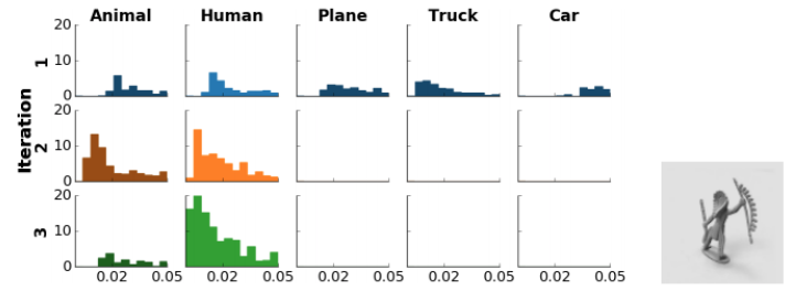
Result
The following is the histogram of distances of votes to the mean of each of the 5 final capsules after each routing iteration. Each distance point is weighted by its assignment probability. With a human image as input, we expect, after 3 iterations, the difference is the smallest (closer to 0) for the human column. (any distances greater than 0.05 will not be shown here.)
The error rate for the Capsule network is generally lower than a CNN model with similar number of layers as shown below.
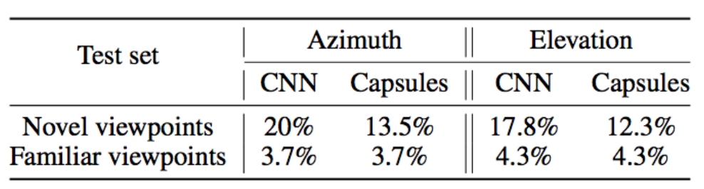
(Source from the Matrix capsules with EM routing paper)
The core idea of FGSM (fast gradient sign method) adversary is to add some noise on every step of optimization to drift the classification away from the target class. It slightly modifies the image to maximize the error based on the gradient information. Matrix routing is shown to be less vulnerable to FGSM adversaries comparing to CNN.
Visualization
The pose matrices in Class Capsules are interpreted as the latent representation of the image. By adjusting the first 2 dimension of the pose and reconstructing it through a decoder (similar to the one in the previous capsule article), we can visualize what the Capsule Network learns for the MNist data.
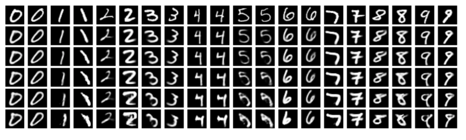
(Source from the Matrix capsules with EM routing paper)
Some digits are slightly rotated or moved which demonstrate the Class Capsules are learning the pose information of the MNist dataset.
Credits
Part of the code implementation in computing the vote and the EM-routing is modified from Guang Yang or Suofei Zhang implementations. Our source code is located at the github. To run,
- Configure the mnist_config.py and cap_config.py according to your environment.
- Run the download_and_convert_mnist.py before running train.py.
Please note that the source code is for illustration purpose with no support at this moment. Readers may refer to other implementations if you have problems to trouble shooting any issues that may come up. Zhang’s implementation seems easier to understand but Yang implementation is closer to the original paper.


 4736
4736


 被折叠的 条评论
为什么被折叠?
被折叠的 条评论
为什么被折叠?
 到【灌水乐园】发言


