场景文本检测算法可微分二值化DBNet原理与代码解析

最新推荐文章于 2024-05-12 11:00:00 发布

00000cj

最新推荐文章于 2024-05-12 11:00:00 发布

阅读量3.6k

点赞数 2

分类专栏：文本检测文章标签：文本检测 DBNet 可微分二值化损失函数后处理

本文链接：https://blog.csdn.net/ooooocj/article/details/112298994

版权

文本检测专栏收录该内容

7 篇文章

订阅专栏

DBNet是一种基于分割的文本检测方法，通过网络学习像素阈值进行二值化，解决了传统固定阈值的局限。文章介绍了其原理，包括概率图与阈值图的标签生成、可微分二值化公式、损失函数（BCE和L1 Loss）以及后处理方法。在后处理阶段，DBNet能直接得到完整文本实例，提高了效率和准确性。

摘要生成于 C知道，由 DeepSeek-R1 满血版支持，前往体验 >

论文 https://arxiv.org/abs/1911.08947

代码 https://github.com/WenmuZhou/DBNet.pytorch

官方解读 https://megvii.blog.csdn.net/article/details/103502283

原理介绍

基于分割的文本检测方法后处理方法通常都是（1）设定固定阈值将分割模型得到的概率图转化为二值图（2）通过一些启发式方法例如像素聚类得到文本实例。本文的创新之处在于将二值化操作嵌入到分割网络中进行联合训练优化，图像中每点的阈值通过网络学习得到，从而把前景像素和背景像素完全区分开。

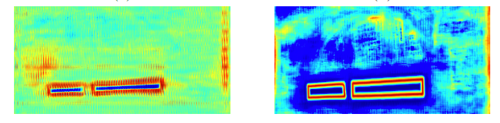
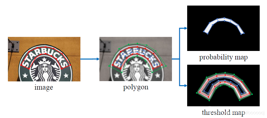
概率图(probability map)和经二值化后的二值图(binary map)共享同一个监督，即文本实例shrink后的kernel，而阈值图的ground truth则是文本实例边界附近区域的像素距离边界的距离，文中说即使没有监督阈值图的输出也会强调边缘信息，如下面左边是无监督的阈值图输出，右边是以边缘信息为监督的阈值图，因此用边缘信息作为阈值图的监督有助于最终的结果。

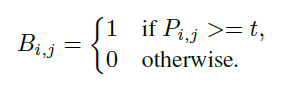
标准的二值化公式如下，其中 $P$ 是概率图， $(i,j)$ 是图中的像素坐标， $t$ 是固定阈值， $B$ 是输出的二值图

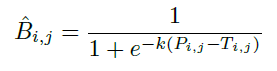
但是标准的二值化不可微，没法和分割网络一起训练优化，因此作者提出了可微分的二值化，公式如下，其中 $T$ 是阈值图， $k$ 取50

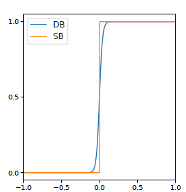
从下图可以看出可微分二值化和标准二值化很相似，且可微分，因此可以和分割网络一起联合优化。

Label Generation

概率图的label和psenet一样，以shrink距离D后的kernel作为标签，具体可以参考psenet。阈值图是文本实例边缘向内shrink距离D到向外expand距离D这个区域内，计算每个像素点到文本边缘的距离作为gt值，距离越近值越大，官方实现中归一化到0.3~0.7之间。生成的标签如下所示，其中红线是文本原始边缘，蓝线是shrink后的边缘，绿线是expand后的边缘

生成阈值图ground truth的代码如下

class MakeBorderMap:
    def __init__(self, shrink_ratio=0.4, thresh_min=0.3, thresh_max=0.7):
        self.shrink_ratio = shrink_ratio  # 0.4
        self.thresh_min = thresh_min  # 0.3
        self.thresh_max = thresh_max  # 0.7

    def __call__(self, data: dict) -> dict:
        """
        :param data: {'img':,'text_polys':,'texts':,'ignore_tags':}
        """
        im = data['img']
        text_polys = data['text_polys']
        ignore_tags = data['ignore_tags']

        canvas = np.zeros(im.shape[:2], dtype=np.float32)
        mask = np.zeros(im.shape[:2], dtype=np.float32)

        for i in range(len(text_polys)):
            if ignore_tags[i]:
                continue
            self.draw_border_map(text_polys[i], canvas, mask=mask)
        canvas = canvas * (self.thresh_max - self.thresh_min) + self.thresh_min  # 归一化到0.3到0.7之内

        data['threshold_map'] = canvas
        data['threshold_mask'] = mask
        return data

    def draw_border_map(self, polygon, canvas, mask):
        polygon = np.array(polygon)  # (4,2)
        assert polygon.ndim == 2
        assert polygon.shape[1] == 2

        polygon_shape = Polygon(polygon)
        if polygon_shape.area <= 0:
            return
        distance = polygon_shape.area * (1 - np.power(self.shrink_ratio, 2)) / polygon_shape.length
        subject = [tuple(l_) for l_ in polygon]

        padding = pyclipper.PyclipperOffset()
        padding.AddPath(subject, pyclipper.JT_ROUND, pyclipper.ET_CLOSEDPOLYGON)

        padded_polygon = np.array(padding.Execute(distance)[0])  # 往外扩
        # padding.Execute结果可能会出现负数
        cv2.fillPoly(mask, [padded_polygon.astype(np.int32)], 1.0)

        xmin = padded_polygon[:, 0].min()
        xmax = padded_polygon[:, 0].max()
        ymin = padded_polygon[:, 1].min()
        ymax = padded_polygon[:, 1].max()
        width = xmax - xmin + 1
        height = ymax - ymin + 1
        # 往外扩大之后的polygon的正的外接矩形

        polygon[:, 0] = polygon[:, 0] - xmin  # 原始的polygon坐标平移到这个正的矩形框内
        polygon[:, 1] = polygon[:, 1] - ymin

        xs = np.broadcast_to(
            np.linspace(0, width - 1, num=width).reshape(1, width), (height, width))
        ys = np.broadcast_to(
            np.linspace(0, height - 1, num=height).reshape(height, 1), (height, width))
        # 以这个正的外接矩形左上角为原点，矩形区域内所有点的横坐标和纵坐标
 
        distance_map = np.zeros((polygon.shape[0], height, width), dtype=np.float32)
        for i in range(polygon.shape[0]):  # 4
            j = (i + 1) % polygon.shape[0]
            absolute_distance = self.distance(xs, ys, polygon[i], polygon[j])
            distance_map[i] = np.clip(absolute_distance / distance, 0, 1)  # 只考虑原始polygon向里外扩distance这个区域
        distance_map = distance_map.min(axis=0)
        # 这一步是限制polygon某条边附近distance区域内的点只取到这条边的距离，而不是到其它边的距离

        xmin_valid = min(max(0, xmin), canvas.shape[1] - 1)
        xmax_valid = min(max(0, xmax), canvas.shape[1] - 1)
        ymin_valid = min(max(0, ymin), canvas.shape[0] - 1)
        ymax_valid = min(max(0, ymax), canvas.shape[0] - 1)
        canvas[ymin_valid: ymax_valid + 1, xmin_valid: xmax_valid + 1] = np.fmax(  # Element-wise maximum of array elements
            1 - distance_map[
                ymin_valid - ymin: ymax_valid - ymax + height,
                xmin_valid - xmin: xmax_valid - xmax + width],
            canvas[ymin_valid: ymax_valid + 1, xmin_valid: xmax_valid + 1])
        # 距离原始polygon越近值越接近1，超出distance的值都为0

    @staticmethod
    def distance(xs, ys, point_1, point_2):
        """
        compute the distance from point to a line
        ys: coordinates in the first axis
        xs: coordinates in the second axis
        point_1, point_2: (x, y), the end of the line
        """
        # height, width = xs.shape[:2]
        square_distance_1 = np.square(xs - point_1[0]) + np.square(ys - point_1[1])
        square_distance_2 = np.square(xs - point_2[0]) + np.square(ys - point_2[1])
        square_distance = np.square(point_1[0] - point_2[0]) + np.square(point_1[1] - point_2[1])

        cosin = (square_distance - square_distance_1 - square_distance_2) / (
                    2 * np.sqrt(square_distance_1 * square_distance_2))
        square_sin = 1 - np.square(cosin)
        square_sin = np.nan_to_num(square_sin)

        result = np.sqrt(square_distance_1 * square_distance_2 * square_sin / square_distance)
        result[cosin < 0] = np.sqrt(np.fmin(square_distance_1, square_distance_2))[cosin < 0]  # 这一步是为什么？
        # self.extend_line(point_1, point_2, result)
        return result