机器学习笔记——梯度下降:

最新推荐文章于 2021-10-11 22:23:07 发布

panghaomingme

最新推荐文章于 2021-10-11 22:23:07 发布

阅读量299

点赞数 1

分类专栏：机器学习

本文链接：https://blog.csdn.net/panghaomingme/article/details/54312972

版权

机器学习专栏收录该内容

25 篇文章 1 订阅

订阅专栏

Andrew Ng教授在机器学习课程里介绍了两种梯度下降的方法：(1)批梯度下降 (2)随机梯度下降（增量梯度下降）

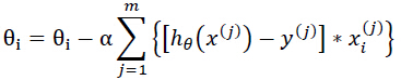
(1)批梯度下降算法

公式：

代码：

clear all;  
close all;  
%批梯度下降
load x.mat;  
load y.mat; 
x=[ones(6,1),x];
n=size(x,2);%特征维数  
m=size(x,1);%样本个数 

alpha=0.001;  
theta=zeros(n,1);%参数初始化为0向量  
for k=1:10000  
    for j=1:m  
        for i=1:n  
            theta(i,1)=theta(i,1)-alpha*(x(j,:)*theta-y(j,1))*x(j,i);  
        end  
    end  
end  
figure;  
plot(x(:,2),y,'r.');%原始数据  
hold on;  
y=theta'*x';%拟合数据  
plot(x(:,2),y);  
for i=1:n  
    fprintf('theta%d=%f;\n',i-1,theta(i,1));%打印估计的参数  
end  
%完

批梯度下降算法的优点是能找到局部最优解，但是若训练样本m很大的话，其每次迭代都要计算所有样本的偏导数的和，时间过慢，于是采用下述另一种梯度下降方法。

随机梯度下降法：

代码：

close all;  
load x.mat;  
load y.mat;  
x=[ones(6,1),x];
figure;  
plot(x(:,2),y,'r.');  
n=size(x,2);%特征维数  
m=size(x,1);%样本个数  
alpha=0.01;%下降速度  
theta=zeros(n,1);%参数  
t=theta;  
for iteration=1:1000%迭代次数  
    for i=1:n  
        t(i,1)=theta(i,1)-alpha*x(:,i)'*(x*theta-y);  
    end  
    theta=t;%同时更新theta值  
end  
figure;  
plot(x(:,2),y,'r.');  
hold on;  
y=theta'*x';  
plot(x(:,2),y);  
for i=1:n  
    fprintf('theta%d=%f;\n',i-1,theta(i,1));%打印估计的参数  
end  
%完