机器学习2

分类算法

1.sklearn转换器和估计器

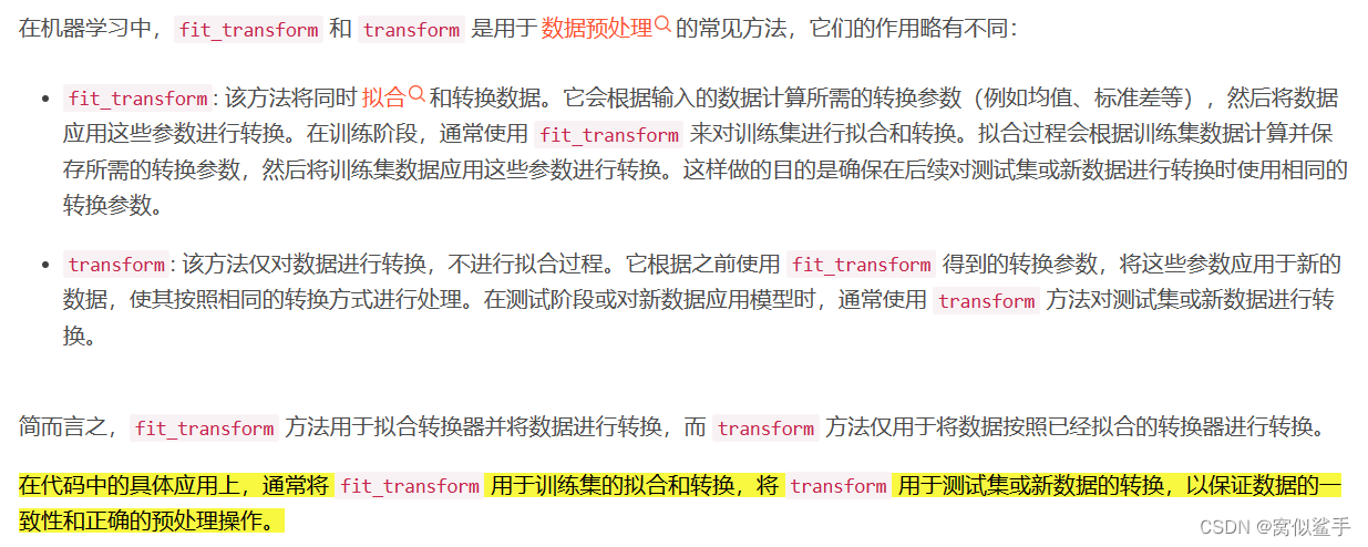
转换器：特征工程父类，  实例化一个转换器（Transformer）

调用fit_transform()

估计器: 实例一个estimator  2. estimator.fit(x_train, y_train) 计算

调用完成，模型生成

3. 模型评估：

1）直接对比真实值和预测值

y_predict =estimator.predict(x_test)

y_test==y_predict

2)计算准确率

accuracy =estimator.score(x_text, y_text)

2.K--近邻算法

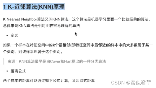
 核心思想：

根据“邻居”判断类别 

计算距离：曼哈顿距离  明可夫斯基距离

 ** k取的过小 容易受到异常点的影响   **  k值过大 样本不均衡的影响

案例1：鸢尾花种类预测

1）获取数据 2）数据集划分 3）特征工程  标准化 4）KNN预估器流程 5）

def knn_demo():
    iris = load_iris()
    x_train, x_text, y_train, y_text = train_test_split(iris.data, iris.target, random_state=6)
    transfer = StandardScaler()
    x_train = transfer.fit_transform(x_train)
    x_text = transfer.transform(x_text)
    estimator = KNeighborsClassifier(n_neighbors=3)
    estimator.fit(x_train, y_train)
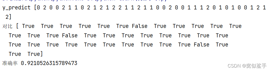
    y_predict = estimator.predict(x_text)
    print("y_predict", y_predict)
    print("对比", y_text == y_predict)
    #计算准确率
    score = estimator.score(x_text, y_text)
    print("准确率", score)

                                x_train 用fit.transform     x_text 用transform

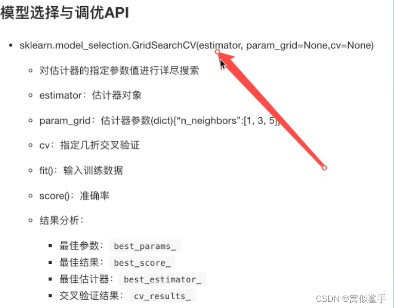
3.模型选择与调优

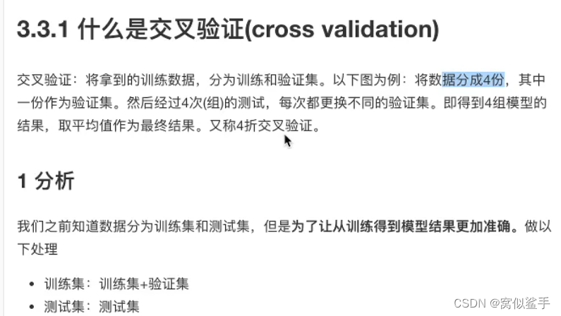
3.1 交叉验证

目的：为了让被评估的模型更加准确可惜

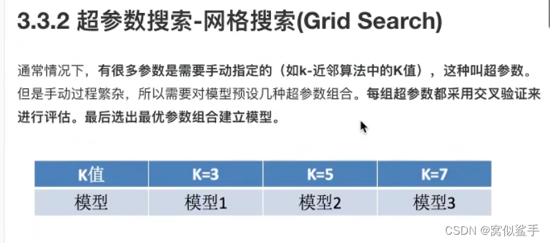
3.2 超参数搜索-网格搜索

K的取值

3.3鸢尾花案列增加K值调优

def knn_demo_gscv():
    iris = load_iris()
    x_train, x_text, y_train, y_text = train_test_split(iris.data, iris.target, random_state=6)
    transfer = StandardScaler()
    x_train = transfer.fit_transform(x_train)
    x_text = transfer.transform(x_text)
    param_grid={"n_neighbors":[1,3,5,7,9,11]}
    estimator = KNeighborsClassifier()
    estimator=GridSearchCV(estimator,param_grid,cv=10)  cv 几折交叉验证

    estimator.fit(x_train, y_train)
    y_predict = estimator.predict(x_text)
    print("y_predict", y_predict)
    print("对比", y_text == y_predict)
    #计算准确率
    score = estimator.score(x_text, y_text)
    print("准确率", score)
    print("最佳参数：\n",estimator.best_params_)
    print("最佳结果：\n", estimator.best_score_)
    print("最佳估计器：\n", estimator.best_estimator_)
    print("交叉验证结果：\n", estimator.cv_results_)
    return None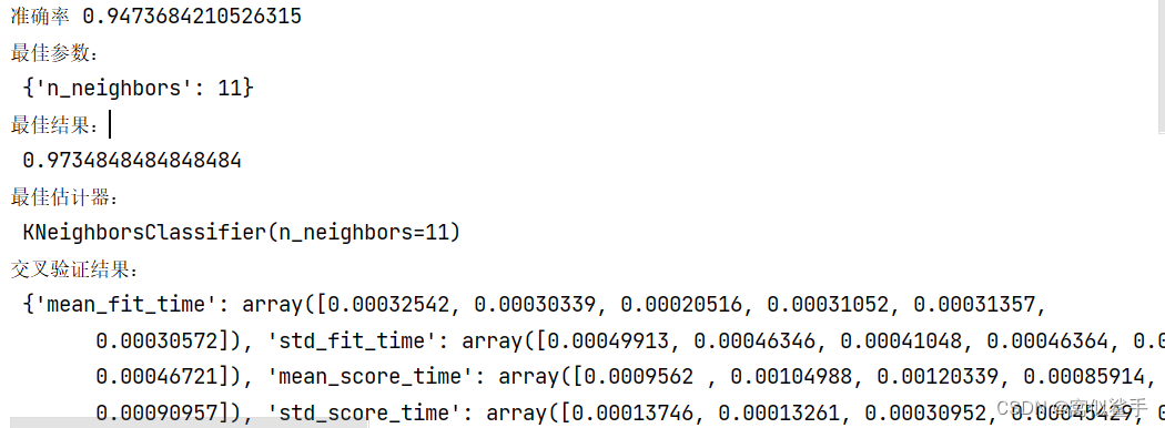

3.4 facebook签到预测 

流程分析：1）获取数据  2）数据处理  目的：特征值x，目标值y  a.缩小数据范围  b.time->年月日时分秒  c. 过滤签到次数少的地点 3）特征工程 4)KNN算法预估流程 模型选择调优 模型评估

import pandas as pd
from sklearn.neighbors import KNeighborsClassifier
from sklearn.preprocessing import StandardScaler
from sklearn.model_selection import train_test_split, GridSearchCV

data=pd.read_csv("D:\\facebook\\FaceBook_train.csv\\FaceBook_train.csv")
#基本数据处理
data=data.query("x<2.5 & x>2 & y>1.0")
#处理时间特征
time_value=pd.to_datetime(data["time"],unit="s")
time=pd.DatetimeIndex(time_value)
data["day"]=time.day
data["weekday"]=time.weekday
data["hour"]=time.hour

place_count=data.groupby("place_id").count()["row_id"]
#print(place_count[place_count>3].head())
data_final=data[data["place_id"].isin(place_count[place_count>3].index.values)]
x=data_final[["x","y","accuracy","day","weekday","hour"]]
y=data_final["place_id"]
#数据集划分

x_train,x_text,y_train,y_text=train_test_split(x,y)
#特征工程：标准化
transfer = StandardScaler()
x_train = transfer.fit_transform(x_train)
x_text = transfer.transform(x_text)

#KNN算法预估器
estimator = KNeighborsClassifier()
#加入网格搜索和交叉验证
#参数准备
param_grid = {"n_neighbors": [1,3, 5,6, 7, 9]}
estimator = GridSearchCV(estimator, param_grid, cv=5)
estimator.fit(x_train, y_train)
#模型评估
#1）直接对比真实值和预测值
y_predict = estimator.predict(x_text)
print("y_predict", y_predict)
print("对比", y_text == y_predict)
# 计算准确率
score = estimator.score(x_text, y_text)
print("准确率", score)
print("最佳参数：\n", estimator.best_params_)
print("最佳结果：\n", estimator.best_score_)
print("最佳估计器：\n", estimator.best_estimator_)
print("交叉验证结果：\n", estimator.cv_results_)

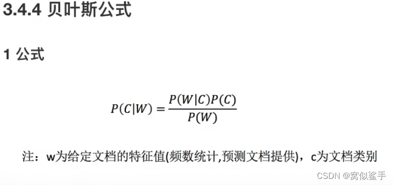
4.朴素贝叶斯算法

联合概率:包含多个条件，且所有条件同时成立的概率 

 条件概率:就是事件A在另外一个事件B已经发生条件下的发生概率

朴素?

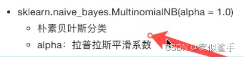
假设:特征与特征之间是相互独立朴素贝叶斯算法:朴素＋贝叶斯应用场景: 文本分类 单词作为特征

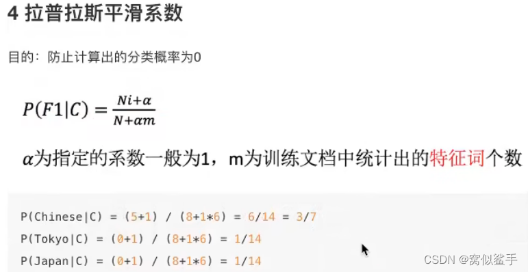
 拉普拉斯平滑系数

 20类新闻分类案例

def nb_news():
    #获取数据集
    news=fetch_20newsgroups(subset="all")
    #划分数据集
    x_train, x_text, y_train, y_text = train_test_split(news.data,news.target)
    #特征工程
    transfer=TfidfVectorizer
    x_train=transfer.fit_transform(x_train)
    x_text=transfer.transform(x_text)
    #朴素贝叶斯算法预估器流程
    estimator=MultinomialNB()
    estimator.fit(x_train,y_train)
    #模型评估
    y_predict = estimator.predict(x_text)
    print("y_predict", y_predict)
    print("对比", y_text == y_predict)
    # 计算准确率
    score = estimator.score(x_text, y_text)
    print("准确率", score)

 

 朴素贝叶斯算法总结

优点：对缺失数据不太敏感，算法也比较简车，常用于文本分类。分类准确度高,速度快

缺点：由于使用了样本属性独立性的假设，所以如果特征属性有关联时其效果

5.决策树

6.集成学习方法之随机森林