


Abstract
Over the past decade, multivariate time series classification has
received great attention. We propose transforming the existing
univariate time series classification models, the Long Short Term
Memory Fully Convolutional Network (LSTM-FCN) and Attention LSTM-FCN (ALSTM-FCN), into a multivariate time series classification model by
augmenting the fully convolutional block with a squeeze-and-excitation
block to further improve accuracy. Our proposed models outperform most
state-of-the-art models while requiring minimum preprocessing. The
proposed models work efficiently on various complex multivariate time
series classification tasks such as activity recognition or action
recognition. Furthermore, the proposed models are highly efficient at
test time and small enough to deploy on memory constrained systems.
在过去的几十年里,多变量时间序列分类问题引起了广泛的关注。我们提出转换现存的单变量时间序列分类模型:长短期记忆全卷积神经网络和注意力LSTM-FCN,转换为多变量时间序列分类模型通过应用挤压-激励块到FCN中去提升准确性。我们提出的模型表现优于最先进的模型,同时需要最少的预处理。这提出的模型在各种复杂的多变量时间上有效工作实现分类任务,如活动识别或操作认可。此外,所提出的模型在测试时十分高效,并且足够小,可以在内存受限的系统上部署。
1.Introduction
Time series data is used in various fields of studies, ranging from
weather readings to psychological signals [1, 2, 3, 4]. A time series
is a sequence of data points in a time domain, typically in a uniform
interval [5]. There is a significant increase of time series data
being collected by sensors [6]. A time series dataset can be
univariate, where a sequence of measurements from the same variable
are collected, or multivariate, where a sequence of measurements from
multiple variables or sensors are collected [7]. Over the past decade,
multivariate time series classification has received significant
interest. Multivariate time series classifications are applied in
healthcare [8], phoneme classification [9], activity recognition,
object recognition, and action recognition [10, 11, 12, 13]. In this
paper, we propose two deep learning models that outperform existing
algorithms.
时间序列被很多研究领域所使用,从天气读数与心理信号。时间序列是时域中的一系列数据点,通常采用统一间隔。
Several time series classification algorithms have been developed
over the years. Distance based methods along with k-nearest neighbors
have proven to be successful in classifying multivariate time series [14]. Plenty of research indicates Dynamic Time Warping (DTW)
as the best distance-based measure to use along k-NN [15].
一些时间序列分类算法在这些年中被开发了出来。基于距离的k近邻算法已经在分类多变量时间序列中取得了成功,大量研究表明动态时间规划 (DTW)是沿 k-NN 使用的最佳基于距离的方法 [15]。
In addition to distance-based metrics, other algorithms are used.
Typically, featurebased classification algorithms rely heavily on the
features being extracted from the time series data [16]. However,
feature extraction is arduous because intrinsic features of time
series data are challenging to capture. For this reason,
distance-based approaches are more successful in classifying
multivariate time series data [17]. Hidden State Conditional Random
Field (HCRF) and Hidden Unit Logistic Model (HULM) are two successful
feature-based algorithms which have led to state-of-the-art results on
various benchmark datasets, ranging from online character recognition
to activity recognition [18]. HCRF is a computationally expensive
algorithm that detects latent structures of the input time series data
using a chain of k-nominal latent variables. The number of parameters
in the model increases linearly with the total number of latent states
required [19]. Further, datasets that require a large number of latent
states tend to overfit the data. To overcome this, HULM proposes using
H binary stochastic hidden units to model 2H latent structures of the
data with only O(H) parameters. Results indicate HULM outperforming
HCRF on most datasets [18]
Traditional models, such as the naive logistic model (NL) and Fisher
kernel learning (FKL) [20], show strong performance on a wide variety
of time series classification problems. The NL logistic model is a
linear logistic model that makes a prediction by summing the inner
products between the model weights and feature vectors over time,
which is followed by a softmax function [18]. The FKL model is
effective on time series classification problems when based on Hidden
Markov Models (HMM). Subsequently, the features or representation from
the FKL model is used to train a linear SVM to make a final
prediction. [20, 21]
传统的模型,比如NL模型在诸多时间序列的分类问题上展现出了很好的性能。NL逻辑模型是一个线性逻辑模型,其通过对内部求和进行预测随时间推移在模型权重和特征向量之间乘积,其后紧跟为softmax函数。
Another common approach for multivariate time series classification is
by applying dimensional reduction techniques or by concatenating all
dimensions of a multivariate time series into a univariate time
series. Symbolic Representation for Multivariate Time Series (SMTS)
[22] applies a random forest on the multivariate time series to
partition it into leaf nodes, each represented by a word to form a
codebook. Every word is used with another random forest to classify
the multivariate time series. Learned Pattern Similarity (LPS) [23] is
a similar model that extracts segments from the multivariate time
series. These segments are used to train regression trees to find
dependencies between them. Each node is represented by a word.
Finally, these words are used with a similarity measure to classify
the unknown multivariate time series. Ultra Fast Shapelets (UFS) [24]
obtains random shapelets from the multivariate time series and applies
a linear SVM or a Random Forest classifier. Subsequently, UFS was
enhanced by computing derivatives as features (dUFS) [24]. The
Auto-Regressive (AR) kernel [25] applies an AR kernel-based distance
measure to classify the multivariate time series. Auto-Regressive
forests for multivariate time series modeling (mv-ARF) [26] uses a
tree ensemble, where the trees are trained with different time lags.
Most recently, WEASEL+MUSE [27] builds a multivariate feature vector
using a classical bag of patterns approach on each variable with
various sliding window sizes to capture discrete features, words, and
pairs of words. Subsequently, feature selection is used to remove
non-discriminative features using a Chi-squared test. The final
classification is obtained using a logistic classifier on the final
feature vector.
Deep learning has also yielded promising results for multivariate time
series classification. In 2014, Yi et al. propose using Multi-Channel
Deep Convolutional Neural Network (MCDCNN) for multivariate time
series classification. MC-DCNN takes input from each variable to
detect latent features. The latent features from each channel are fed
into an MLP to perform classification [17]. This paper proposes two
deep learning models for multivariate time series classification.
These proposed models require minimal preprocessing and are tested on
35 datasets, obtaining strong performances in most of them.
Performance is the classification accuracy of a model on a particular
dataset. The rest of the paper is ordered as follows. Background works
are discussed in Section 2. We present the architecture of the two
proposed models in Section 3. In Section 4, we discuss the dataset,
evaluate the models on them, present our results and analyze our
findings. In Section 5, we draw our conclusion.
2.Background Works
2.1Recurrent Neural Networks
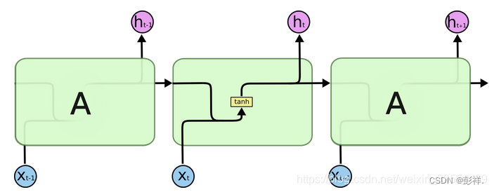
Recurrent Neural Networks (RNN) are a form of neural networks that
display temporal behavior through the direct connections between
individual layers. Pascanu et al. [28] implement RNN to maintain a
hidden vector h that is updated at time step t,
递归神经网络(RNN)是一种神经网络模型,它通过各个层之间的直接联系来展示时间行为。隐藏层向量 h 在每个时间步长 t 内更新,
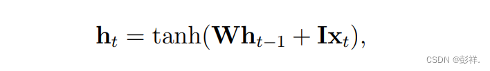
where the hyperbolic tangent function is represented by tanh, the
input vector at time step t is denoted as xt , the recurrent weight
matrix is denoted by W and the projection matrix is signified by I. A
prediction, yt can be made using a hidden state, h, and a weight
matrix, W,
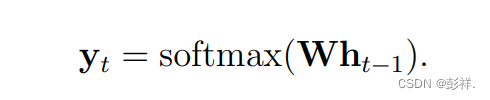
其中双曲切函数由 tanh 表示,在每个时间步长t内的输入向量用x表示,回归权重矩阵用W表示,投影矩阵用I表示。结果y可有W与h的内积再使用Softmax函数获得。
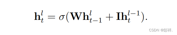
The softmax function normalizes the output predictions of the model to
be a valid probability distribution and the logistic sigmoid function
is declared as σ. RNNs can be stacked to create deeper networks by
using the hidden state, h l−1 of a RNN layer l−1 as an input to the
hidden state, h l of another RNN layer l,
softmax函数将模型的输出预测归一化为是有效的概率分布和逻辑 sigmoid 函数被声明为σ。RNN 可以通过以下方式堆叠以创建更深层次的网络使用隐藏状态,RNN 层 l−1 的 h l−1 作为隐藏状态,另一个RNN层的h l,
2.2Long Short-Term Memory RNN
A major issue with RNNs is that they often have to face the issue of
vanishing gradients. Long short-term memory (LSTM) RNNs address this problem by integrating gating functions into their state dynamics
[29]. An LSTM maintains a hidden vector, h, and a memory vector, m,
which control state updates and outputs at each time step,
respectively.The computation at each time step is depicted by Graves et al. [30] as the following:
RNN需要面对的一个问题是梯度消失。LSTM通过将门控函数来动态修改来解决此问题。LSTM包含一个隐藏向量h一个记忆向量m,它控制在每个时间步长中的状态更新。计算公式如下:
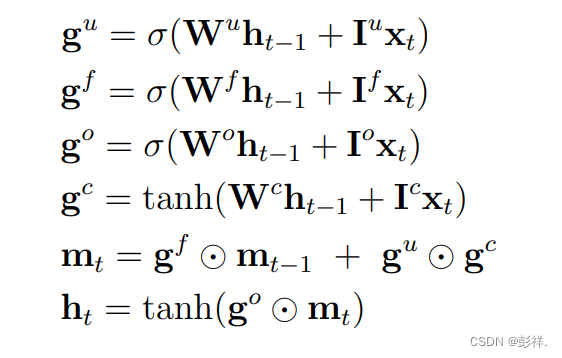
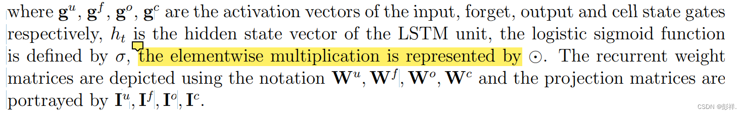
这里 gu, gf, go, gc分别代表输入向量,记忆单元,输出向量和细胞状态,ht是LSTM单元的隐藏向量,somtmax函数由 σ 代表。回归权重矩阵分别使用 Wu,Wf ,Wo,Wc 来表示。
LSTMs can learn temporal dependencies. However, long-term dependencies of long sequence are challenging to learn using LSTMs. Bahdanau et al. [31] proposed using an attention mechanism to learn these long-term dependencies.
LSTMs能够学习短期依赖,然而,使用 LSTM 很难学习长序列的长期依赖性。Bahdanau 提出了注意力机制去学习长序列依赖。
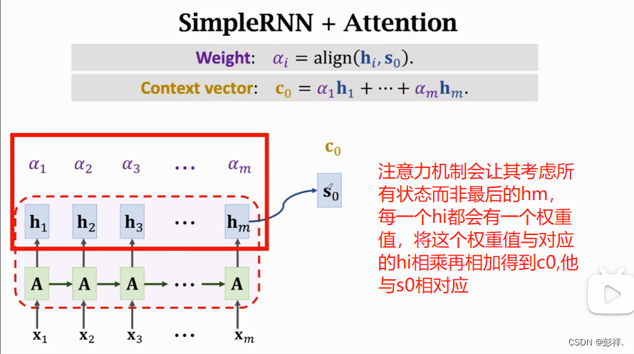
2.3Attention Mechanism
An attention mechanism conditions a context vector V on the target
sequence y. This method is commonly used in neural translation of
texts. Bahdanau et al.[31] argues the context vector vi depends on a
sequence of annotations (b1, …, bTx), of length Tx which is the
maximum length of the input sequence x, where an encoder maps the
input sequence. Each annotation, bi, comprises information on the
whole input sequence, while focusing on regions surrounding the i-th
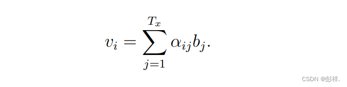
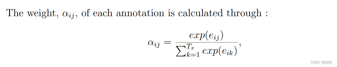
word of the input sequence. The weighted sum of each annotation, bi,is
used to compute the context vector as follows:
注意机制应用了一个上下文向量V到目标序列y上,这种方法通常用于翻译文本,Bahdanau认为上下文向量 Vi 取决于注释序列。
3 Multivariate LSTM Fully Convolutional Network
3.1Network Architecture
Long Short Term Memory Fully Convolutional Network (LSTM-FCN) and
Attention LSTM-FCN (ALSTM-FCN) have been successful in classifying
univariate time series [33]. However, they have never been applied to
on a multivariate time series classification problem. The models we
propose, Multivariate LSTM-FCN (MLSTM-FCN) and Multivariate Attention
LSTM-FCN (MALSTM-FCN), converts their respective univariate models
into multivariate variants. We extend the squeeze-and-excite block to
the case of 1D sequence models and augment the fully convolutional
blocks of the LSTM-FCN and ALSTM-FCN models to enhance classification
accuracy.
长短期记忆全卷积神经网络以及注意力-LSTM-FCN在单变量时间序列分类中已经取得了成功。然而,它们从未应用到多变量时间序列分类问题中。我们提出的:多变量LSTM_FCN以及多变量注意力LSTM-FCN,将它们各自的单变量模型转换为多变量变体。我们将挤压和激励块扩展到一维序列模型,增强了LSTM-FCN中的全卷积块,以加强分类准确性。
As the datasets now consist of multivariate time series, we can define
a time series dataset as a tensor of shape (N, Q, M ), where N is the
number of samples in the dataset, Q is the maximum number of time
steps amongst all variables and M is the number of variables processed
per time step. Therefore a univariate time series dataset is a special
case of the above definition, where M is 1. The alteration required to
the input of the LSTM-FCN and ALSTM-FCN models is to accept M inputs
per time step, rather than a single input per time step.
因为数据集目前由多变量时间序列组成,我们定义一个时间序列为一个形状为(N,Q,M)的tensor,N 是数据集中的样本数,Q 是在所有变量之间的步长的最大数目,M 是每个时间步长中被处理的变量的个数。因此,一个单变量时间序列数据集是上面定义中的一个特殊例子,它的M为1。这个调整要求LSTM-FCN和ALSTM-FCN的输入要去在每个步长接收M个输入,而不是每个步长单个输入
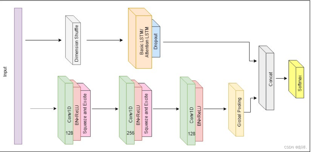
Similar to LSTM-FCN and ALSTM-FCN, the proposed models comprise a fully convolutional block and a LSTM block, as depicted in Fig. 1. The fully convolutional block contains three temporal convolutional blocks, used as a feature extractor, which is replicated from the original fully convolutional block by Wang et al [34]. The convolutional blocks contain a convolutional layer with a number of filters (128, 256, and 128) and a kernel size of 8, 5, and 3 respectively. Each convolutional layer is succeeded by batch normalization, with a momentum of 0.99 and epsilon of 0.001. The batch normalization layer is succeeded by the ReLU activation function. In addition, the first two convolutional blocks conclude with a squeeze-and-excite block, which sets the proposed model apart from LSTM-FCN and ALSTM-FCN. Fig. 2 summarizes the process of how the squeeze-and-excite block is computed in our architecture. For all squeeze and excitation blocks, we set the reduction ratio r to 16. The final temporal convolutional block is followed by a global average pooling layer.
与LSTM-FCN和ALSTM-FCN类似,提出的模型包含全卷积块和LSTM块,如上图。全卷积块包含三个时间卷积块,作为特征提取器。卷积块包含分别包含128,256,128个卷积核,大小分别为8,5,3.每个卷积层后紧跟批量归一化,设置动量为0.99,舍入误差为0.001(是指运算得到的近似值和精确值之间的差异)。批归一化层后紧跟的是ReLU激活函数。此外,在前两个卷积层中还包含一个挤压-激励块,它是所提出的LSTM-FCN和ALSTM-FCN的一部分,下图为该模块的在本结构中的计算过程,对于整个挤压-激励模块,我们设置减速比r为16,最后时序卷积块后为一个平均池化层。如上图所示。
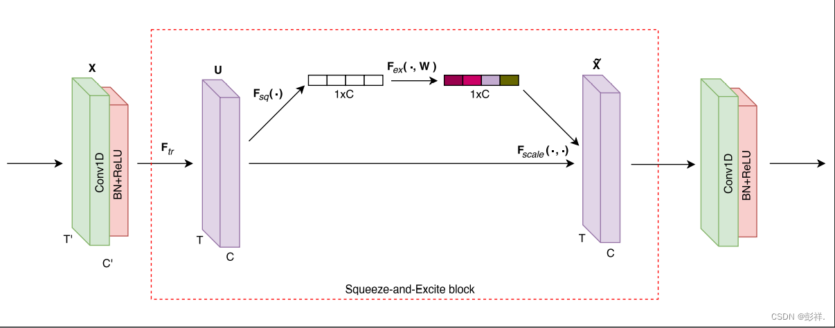
The squeeze-and-excite block is an addition to the FCN block which
adaptively recalibrates the input feature maps. Due to the reduction
ratio r set to 16, the number of parameters required to learn these
self-attention maps is reduced such that the overall model size
increases by just 3-10 %. This can be computed as below:
挤压-激励块是对FCN块的补充,其自适应地重新校准输入特征图。(即能够使有效的feature map的权重大,无效或效果小的feature map权重小),由于 r 设置为16,用来学习这些 自-注意力 图的参数数量被减少,使得整体模型大小仅增加了3-10%。
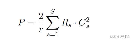
where P is the total number of additional parameters, r denotes the
reduction ratio, S denotes the number of stages (each stage refers to
the collection of blocks operating on feature maps of a common spatial
dimension), Gs denotes the number of output feature maps for stage s
and Rs denotes the repeated block number for stage s. Since the FCN
blocks are kept consistent for all models, we can directly compute the
additional number of parameters as P =2/16 ∗ (1282 + 2562) = 10240
for all models. Squeeze and excitation is essential to the enhanced
performance on multivariate datasets, as not all feature maps may
impact the subsequent layers to the same degree. This adaptive
recalibration of the feature maps can be considered as a form of
learned self-attention on the output feature maps of prior layers.
This adaptive rescaling of the filter maps is of utmost importance to
the improved performance of the MLSTM-FCN model compared to LSTM-FCN,
as it incorporates learned self-attention to the inter-correlations
between multiple variables at each time step, which was inadequate
with the LSTM-FCN.
P是额外参数的总数量,r代表减速比,S代表阶段的数量(每个阶段都是指在公共空间维度的特征地图上运行的块的集合)
In addition, the multivariate time series input is passed through a
dimension shuffle layer (explained more in Section 3.2), followed by
the LSTM block. The LSTM block is identical to the block from the
LSTM-FCN or ALSTM-FCN models [33], comprising either an LSTM layer or
an Attention LSTM layer, which is followed by a dropout layer.
此外,多变量时间序列输入还经过了一个维度混洗,在LSTM块之前。这个LSTM块来自于LSTM或ALSTM模型,由LSTM层或ALSTM层组成,之后是丢失层。
3.2动量(momentum)
在普通的梯度下降法x += v中,每次x的更新量v为v = - dx * lr,其中dx为目标函数func(x)对x的一阶导数,。
当使用冲量时,则把每次x的更新量v考虑为本次的梯度下降量- dx * lr与上次x的更新量v乘上一个介于[0,
1]的因子momentum的和,即v = - dx * lr + v * momemtum。 从公式上可看出:
- 当本次梯度下降- dx * lr的方向与上次更新量v的方向相同时,上次的更新量能够对本次的搜索起到一个正向加速的作用。
- 当本次梯度下降- dx * lr的方向与上次更新量v的方向相反时,上次的更新量能够对本次的搜索起到一个减速的作用。
import numpy as np
import matplotlib.pyplot as plt


# 目标函数:y=x^2
def func(x):
    return np.square(x)

# 目标函数一阶导数:dy/dx=2*x
def dfunc(x):
    return 2 * x

def GD_momentum(x_start, df, epochs, lr, momentum):
    """
    带有冲量的梯度下降法。
    :param x_start: x的起始点
    :param df: 目标函数的一阶导函数
    :param epochs: 迭代周期
    :param lr: 学习率
    :param momentum: 冲量
    :return: x在每次迭代后的位置(包括起始点),长度为epochs+1
    """
    xs = np.zeros(epochs+1)
    x = x_start
    xs[0] = x
    v = 0
    for i in range(epochs):
        dx = df(x)
        # v表示x要改变的幅度
        v = - dx * lr + momentum * v
        x += v
        xs[i+1] = x
    return xs
为了查看momentum大小对不同学习率的影响,此处设置学习率为lr = [0.01, 0.1, 0.6, 0.9],冲量依次为momentum = [0.0, 0.1, 0.5, 0.9],起始位置为x_start = -5,迭代周期为6。测试以及绘图代码如下:
def demo2_GD_momentum():
    line_x = np.linspace(-5, 5, 100)
    line_y = func(line_x)
    plt.figure('Gradient Desent: Learning Rate, Momentum')

    x_start = -5
    epochs = 6

    lr = [0.01, 0.1, 0.6, 0.9]
    momentum = [0.0, 0.1, 0.5, 0.9]

    color = ['k', 'r', 'g', 'y']

    row = len(lr)
    col = len(momentum)
    size = np.ones(epochs+1) * 10
    size[-1] = 70
    for i in range(row):
        for j in range(col):
            x = GD_momentum(x_start, dfunc, epochs, lr=lr[i], momentum=momentum[j])
            plt.subplot(row, col, i * col + j + 1)
            plt.plot(line_x, line_y, c='b')
            plt.plot(x, func(x), c=color[i], label='lr={}, mo={}'.format(lr[i], momentum[j]))
            plt.scatter(x, func(x), c=color[i], s=size)
            plt.legend(loc=0)
    plt.show()
运行结果如下图所示,每一行的图的学习率lr一样,每一列的momentum一样,最左列为不使用momentum时的收敛情况:
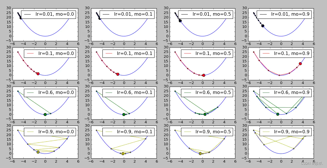
简单分析一下运行结果:
- 从第一行可看出:在学习率较小的时候,适当的momentum能够起到一个加速收敛速度的作用。
- 从第四行可看出:在学习率较大的时候,适当的momentum能够起到一个减小收敛时震荡幅度的作用。
3.3批量归一化(BatchNormalization)
为何要使用BN呢?
机器学习领域有个很重要的假设:IID独立同分布假设【数据的独立同分布(Independent Identically Distributed)】————假设训练数据和测试数据是满足相同分布的,这是通过训练数据获得的模型能够在测试集获得好的效果的一个基本保障。如果训练数据与测试数据的分布不同,那么网络的泛化能力就会大大降低。另一方面,如果每批训练数据的分布各不相同,网络就要在每次迭代时都去学习适应不同的分布,那么网络的训练速度就会大大降低,这就是为什么我们需要对输入数据做一个归一化处理。
近年来深度学习异常火爆,并且在视觉、语音和其他诸多领域屡创佳绩,随机梯度下降(SGD)成了训练深度神经网络的主流方法。虽然SGD对于训练深度神经网络来说是简单高效的,但它被人诟病的地方是,需要对模型的超参数进行仔细地选择,比如:权重衰减系数、Dropout比例、特别是优化中使用的学习率以及模型的参数初始化。
由于每个层的输入都受到前面所有层的参数影响,因此,当网络变得更深时,网络参数的微小变化也会被逐渐放大,这使得训练变得越来越复杂,收敛越来越慢。这是一个深度学习领域的接近本质的问题,已经有很多论文提出了解决方法,比如:
RELU激活函数,ResidualNetwork残差网络等等。BN本质上也是其中一种目前被大量使用的解决方法。
BN是一个深度神经网络的训练技巧,它不仅可以加快了模型的收敛速度,而且更重要的是在一定程度缓解了深层网络中“梯度弥散”的问题,从而使得深层网络模型的训练更加容易和稳定。
从字面意思看来Batch Normalization(简称BN)就是对每一批数据进行归一化,确实如此,对于训练中某一个batch的数据{x1,x2,…,xn},注意这个数据是可以输入也可以是网络中间的某一层输出。在BN出现之前,我们的归一化操作一般都在数据输入层,对输入的数据进行求均值以及求方差做归一化,但是BN的出现打破了这一个规定,我们可以在网络中任意一层进行归一化处理,因为我们现在所用的优化方法大多都是min-batch SGD,所以我们的归一化操作就成为Batch Normalization。
BN的优点:
- 使得模型训练收敛的速度更快
- 模型隐藏输出特征的分布更稳定,更利于模型的学习
3.4 Network Input
Depending on the dataset, the input to the fully convolutional block and LSTM block vary. The input to the fully convolutional block is a multivariate variate time series with Q time steps having M distinct variables per time step. If there is a time series with M variables and Q time steps, the fully convolutional block will receive the data as such. Variables are defined as the channels of interconnected data streams.
取决于数据集,全卷积块和 LSTM 块的输入变化。全卷积块的输入是多变量时间序列,包含Q个时间步长,每个步长M个不同的向量。如果存在具有 M 个变量和 Q 个时间步长的时间序列,则完全卷积块将接收这样的数据。变量被定义为互连数据流的通道。
In addition, the input to the LSTM can vary depending on the application of dimension shuffle. The dimension shuffle transposes the temporal dimension of the input data. If the dimension shuffle
operation is not applied to the LSTM path, the LSTM will require Q time steps to process M variables at each time step. However, if the dimension shuffle is applied, the LSTM will require M time steps to process Q variables per time step. In other words, the dimension shuffle improves the efficiency of the model when the number of variables M is less than the number of time steps Q.
此外,LSTM的输入能够变化取决于维度混洗的应用。维度混洗转换输入数据的时序维度。如果维度混洗操作没有应用到LSTM中,LSTM将需要Q时间步长来处理每个时间步的M个变量。然而,如果维度混洗被应用,LSTM将需要M个时间步长去处理每个步长Q个变量。总之,维度混洗提高了模型的效率当变量M的数量少于时间步长Q的数量时。
After the dimension shuffle, at each time step t, where 1 ≤ t ≤ M, M being the number of variables, the input provides the LSTM the entire history of that variable (data of that variable over all Q time
steps). Thus, the LSTM is given the global temporal information of each variable at once. As a result, the dimension shuffle operation reduces the computation time of training and inference without losing accuracy for time series classification problems. An ablation test is performed to show the performance of a model with the dimension shuffle operation is statistically the same as a model without using it (further discussed in Section 4.4)
在维度混洗后,在每一个时间步长t,其中1<=t<=M,M作为变量的数码,他的输入为LSTM提供了该变量的整个历史数据(该变量在所有Q时间的数据)。因此,LSTM被一次赋予每个变量的全局时间信息。结果,维度混洗操作在不损失准确性的情况下减少了在时间序列分类问题中的训练和验证的计算时间。有一个消融实验(即控制变量对比实验)展示了拥有维度混洗和没有用到维度混洗的两个模型的性能差距。这将在下面讲到。
The proposed models take a total of 13 hours to process the MLSTM-FCN and a total of 18 hours to process the MALSTM-FCN on a single GTX 1080 Ti GPU. While the time required to train these models is significant, one can note their inference time is comparable with other standard models.
这个模型使用一个 GTX 1080 Ti GPU花费了13个小时去执行MLSTM-FCN,花费了18个小时去执行MALSTM-FCN模型。虽然训练这些模型所需的时间很长,但可以注意到它们的推理时间与其他标准模型相当。
4.Experiments
MLSTM-FCN and MALSTM-FCN have been tested on 35 datasets, in Section
4.2. The optimal number of LSTM cells for each dataset was found via grid search over 3 distinct choices - 8, 64 or 128, and all other hyper parameters are kept constant. The FCN block is comprised of 3 blocks of 128-256-128 filters for all models, with kernel sizes of 8, 5, and 3 respectively, comparable with the original models proposed by Wang et al [34]. Additionally, the first two FCN blocks are succeded by the squeeze-and-excitation block. We consistently chose 16 as the
reduction ratio r for all squeeze-and-excitation blocks, as suggested by Hu et al [32]. During the training phase, we set the total number of training epochs to 250 unless explicitly stated and the dropout rate is set to 80% to mitigate overfitting. Each of the proposed models is trained using a batch size of 128. The convolution kernels are initialized by the Uniform He initialization scheme proposed by He et al [35], which samples from the uniform distribution U ∈, where d is the number of input units to the weight tensor. For datasets with class imbalance, a class weighing scheme inspired by King et al. is utilized [36], weighing the contribution of each class Ci (1 ≤ i ≤ C) to the loss by the factor Gwi =NC×NCi, where Gwi is the loss scaling weight for the i-th class, N is the number of samples in the dataset, C is the number of classes and NCi is a the number of samples which
belong to class Ci.
MLSTM-FCN和MALSTM-FCN曾在35个数据集上测试,通过网格搜索找到每个数据集的最佳 LSTM 单元格数,包括 3 个不同的选项 :8、64 或 128 个,所有其他超参数保持不变。FCN块由3个块组成,分别包含128,256,128个过滤器(卷积核),大小分别为8,5,3(此次为一维卷积层,即为81,51,3*1)。此外,前两个FCN块后紧跟着挤压-激励块。我们持续在挤压-激励块选择16作为减速比。在训练阶段,我们将训练 epoch 的总数设置为 250,除非明确说明,并且辍学率设置为 80% 以减轻过度拟合。每个模型的批次大小都设置为128。
We use the Adam optimizer [37], with an initial learning rate set to
1e-3 and the final learning rate set to 1e-4 to train all models. In
addition, after every 100 epochs, the learning rate is reduced by a
factor of 1/ 2 3 \sqrt[3]{2} 32. The datasets were normalized and
preprocessed to have zero mean and unit variance. We append variable
length time series with zeros afterwards to obtain a time series
dataset with a constant length Q, where Q is the maximum length of the
time series. Mean-standard deviation normalization and zero padding
are the only preprocessing steps performed for all models. We compute
the mean and standard deviation of the training dataset and apply
these values to normalize both the train and test datasets. We use the
Keras [38] library with the Tensorflow backend [39] to train the
proposed models. .
我们使用Adam优化器,初始学习率设置为1e-3,最终学习率设置为1e-4去训练所有模型。此外,美经过100次迭代后,学习率减少为系数的1/ 2 3 \sqrt[3]{2} 32。数据集被归一化,并且预处理为均值和单位方差为零。我们附加变量长度的时间序列,之后使用零来获得时间序列具有恒定长度 Q 的数据集,其中 Q 是时间序列。
The two proposed models attain state-of-the-art results in most of the
datasets tested, 28 out of 35 datasets. Each of the proposed models
requires minimal preprocessing and feature extraction. Furthermore,
the addition of the squeeze-and-excitation block improves the
performance of LSTM-FCN and ALSTM-FCN significantly. We provide a
comparison of our proposed models to other existing state-of-the-art
algorithms.
提出的两个模型在大部分的数据集中取得了先进的成果,35个里面的28个数据集。每个提出的模型需要最少的预处理和特征提取。此外,激励-挤压块显著提高了LSTM-FCN和ALSTM-FCN的性能。我们将这个模型与许多先进的算法做了比较。
The proposed models will be beneficial in various multivariate time
series classification tasks, such as activity recognition, or action
recognition. The proposed models can quickly be deployed in real-time
systems and embedded systems because the proposed models are small and
efficient. Further research is being done to better understand why the
squeeze-and-excitation block does not match the performance of the
general LSTM-FCN or ALSTM-FCN models on a couple of datasets.
该模型将有利于多变量时间序列分类任务,比如活动识别。提出的模型可以快速实时部署系统和嵌入式系统,因为所提出的模型很小,并且高效。正在进行进一步的研究,以更好地了解为什么
挤压和激励模块的性能在一些数据集上的性能并不显著。


 337
337


 被折叠的 条评论
为什么被折叠?
被折叠的 条评论
为什么被折叠?
 到【灌水乐园】发言


