numpy教程：统计函数Statistics

lz总结的一般统计函数

np.unique()

返冋其参数数组中所有不同的值，并且按照从小到大的顺序排列。它有两个可选参数：
return_index : Ture表示同时返回原始数组中的下标。
Return_inverse: True表示返冋重建原始数组用的下标数组。

a = np.array([1, 1, 9, 5, 2, 6, 7, 6, 2, 9])
>>> np.unique(a)
array([l, 2, 5, 6, 7, 9])
>>> x, idx = np.unique(a, return_index=True)
>>> idx
array([0, 4, 3, 5, 6, 2])
>>> a[idx]
array([1, 2, 5, 6, 7, 9])
>>> x, ridx = np.unique(a, return_inverse=True)
>>> ridx
array([0, 0, 5, 2, 1, 3, 4, 3, 1, 5])
>>>all(x[ridx]==a) #原始数组a和x[ridx]完全相同
True

皮皮Blog

Statistics

Order statistics顺序统计量

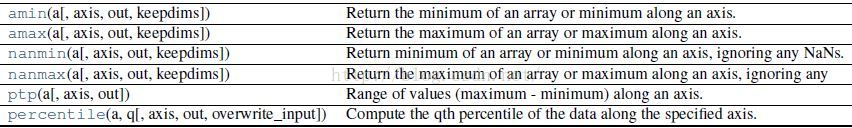
Averages and variances均值和方差

median(a[, axis, out, overwrite_input, keepdims])	Compute the median along the specified axis.
average(a[, axis, weights, returned])	Compute the weighted average along the specified axis.
mean(a[, axis, dtype, out, keepdims])	Compute the arithmetic mean along the specified axis.
std(a[, axis, dtype, out, ddof, keepdims])	Compute the standard deviation along the specified axis.
var(a[, axis, dtype, out, ddof, keepdims])	Compute the variance along the specified axis.
nanmedian(a[, axis, out, overwrite_input, ...])	Compute the median along the specified axis, while ignoring NaNs.
nanmean(a[, axis, dtype, out, keepdims])	Compute the arithmetic mean along the specified axis, ignoring NaNs.
nanstd(a[, axis, dtype, out, ddof, keepdims])	Compute the standard deviation along the specified axis, while ignoring NaNs.
nanvar(a[, axis, dtype, out, ddof, keepdims])	Compute the variance along the specified axis, while ignoring NaNs.

[ numpy教程- 函数库和ufunc函数 ]

Correlating相关

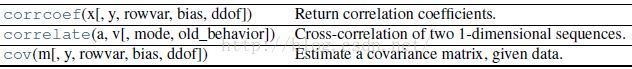
Note: 要实现估计量的无偏性，numpy中的方差计算是除以N，而协方差计算是除以N-1，所以会发现单独计算向量的方差并不会与计算两个向量的协方差矩阵对角线上的元素相等！

a= [0, 1, 2]
print(np.var(a) * 3 == np.cov(a) * 2, '\n')

输出：
True 

当然可以设置度参数bias : int, optional来改变这种计算模式
Default normalization is by (N - 1), where N is the number of observations given (unbiased estimate). If bias is 1, then normalization is by N. These values can be overridden by using the keyword ddof in numpy versions >= 1.5.

Histograms

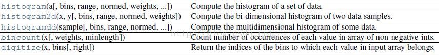
np.histogram()

对一维数组进行直方图统计，其参数列表如下：
Histogram(a,bins=10,range=None,normed=False,weights=None)
其中，a是保存待统计数据的数组，bins指定统计的区间个数，即对统计范围的等分数。 range是一个长度为2的元组，表示统计范围的最小值和最大值，默认值为None,表示范围由 数据的范围决定，即(a.min(), a.max()).当normed参数为False时，函数返回数组a中的数据在每个区间的个数，否则对个数进行正规化处理，使它等于每个区间的概宇密度。weights参数和 bincount()的类似。
NumPy中histogram函数应用到一个数组返回一对变量：直方图数组和箱式向量，即两个一维数组--hist和bin_edges,第一个数组是每个区间的统计结果， 第二个数组长度为len(hist)+1,每两个相邻的数值构成一个统计区间。

Note： matplotlib也有一个用来建立直方图的函数(叫作hist,正如matlab中一样)，与NumPy主要的差别是pylab.hist自动绘制直方图，而numpy.histogram仅仅产生数据。
>>> a = np. random.rand (100)
>>> np.histogram(a,bins=5,range=(0,1))
(array([20,26,20,16,18]), array([ 0. , 0.2, 0.4, 0.6, 0.8, 1.])
如果需要统计的区间长度不等，可以将表示区间分隔位置的数组传递给bins参数:
>>> np.histogram(a,bins=[0, 0.4, 0.8, 1.0], range=(0,1))
(array([46, 36, 18]), array([ 0. , 0.4, 0.8, 1.]))
用weights参数指定了数组a中每个元素对应的权值，那么histogram()将对区间中数 值对应的权值进行求和。

统计男青少年年龄和身高的例子:

sums是每个年龄段的身高总和，cnts是每个年龄段的数据个数，因此很容易计算出每个年龄段的平均身高

>>> sums = np.histogram(d[:,0]，bins=range(7,21)，range=(7,20)，weights=d[:,1])[0]
>>> cnts =np.histogram (d[:,0], bins=range(7,21), range=(7,20))[0]
>>>sums/cnts
array([ 125.96,  132.06666667, 137.82857143, 143.8 ,
148. 14 ,153.44, 162.15555556, 166.86666667, 172.83636364, 173.3,175.275, 174.19166667,175.075])

hist转换成plot折线图

plt.hist直接绘制数据是hist图

plt.hist(z, bins=500, normed=True)

hist图转换成折线图

cnts, bins = np.histogram(z, bins=500, normed=True)
bins = (bins[:-1] + bins[1:]) / 2
plt.plot(bins, cnts)

[matplotlib绘图实例 pyplot、pylab模块及作图参数:hist]

Note: lz建议使用seaborn.distplot()。

np.bincount()

对整数数组中各个元素出现的次数进行统计，它要求数组中所有元素都是非负的。其返回数组中第i个元素的值表示整数i在参数数组中出现的次数。
>>> np.bincount(a)
array([0, 2, 2, 0, 0, 1, 2, 1, 0, 2])
由上面的结果可知,在数组a中有两个1、两个2、一个5、两个6、一个7和两个9,而 0、3、4、8等数没有在数组a中出现。
当指定weights参数时，bincount(x, weights=w)返冋数组x中每个整数所对应的w中的权值之和。
>>> x =np.array([0 , 1, 2, 2, 1, 1, 0])
>>> w = np.array([0.1, 0.3, 0.2,0.4,0.5,0.8,1.2])
>>> np.bincount(x, w)
array ([ 1.3,1.6,0.6])
要求平均值:
>>> np.bincount(x,w)/np.bincount(x)
array([ 0.65 , 0.53333333, 0.3])

但是np.ndarray怎么统计数组每个元素出现的个数呢？

list.count(element)

只能先将np.array.tolist()转换成Python list，再使用list的count方法计数某个元素出现次数。

>>> a = ['a', 'b', 'c', 3, '4', '2', '2', 2, 2]
>>> a.count(2)
2

[python入门教程、基础知识、基本类型的操作及转换 ]

[numpy-ref-1.8.1 : 3.30 Statistics p1256]

[numpy/reference/routines.statistics]

皮皮Blog

统计函数cov协方差矩阵计算示例

空间中有三个点，值得注意的是，这三个点是随机变量的观测值，而坐标系x,y（维度）是随机变量！也就是有N个点，这N个点就是观测值，而每个点有K维，K就是随机变量个数！！！

Consider two variables, x0 and x1, which correlate perfectly, but in opposite directions:
>>> x = np.array([[0, 2], [1, 1], [2, 0]]).T
>>> x
array([[0, 1, 2],
[2, 1, 0]])

Note how x0 increases while x1 decreases. The covariance matrix shows this clearly:
>>> np.cov(x)
array([[ 1., -1.],
[-1., 1.]])
Note that element C0;1, which shows the correlation between x0 and x1, is negative.

Further, note how x and y are combined:
>>> x = [-2.1, -1, 4.3]
>>> y = [3, 1.1, 0.12]
>>> X = np.vstack((x,y))
>>> print np.cov(X)
[[ 11.71 -4.286 ]
[ -4.286 2.14413333]]
>>> print np.cov(x, y)
[[ 11.71 -4.286 ]
[ -4.286 2.14413333]]
>>> print np.cov(x)
11.71
3.30.

Note: 

1. 上面的X等价于np.array([[-2.1, -1, 4.3], [3, 1.1, 0.12]])

2.  从这里可以看出，cov函数的输入可以是矩阵（二维向量），计算的是矩阵中行向量（R.V.）间的协方差矩阵，其对角线上的元素分别是单个行向量（R.V.）的方差。所以如果初始数据[[0, 2], [1, 1], [2, 0]]是观测值要先转置再求协方差！

3. 矩阵的协方差矩阵的计算等价于单独将不同R.V.分量拿出来作为多个参数输入到cov函数中的协方差。

from: http://blog.csdn.net/pipisorry/article/details/48770785

ref: