简单的Tensorflow(7)：tensorboard的简单使用

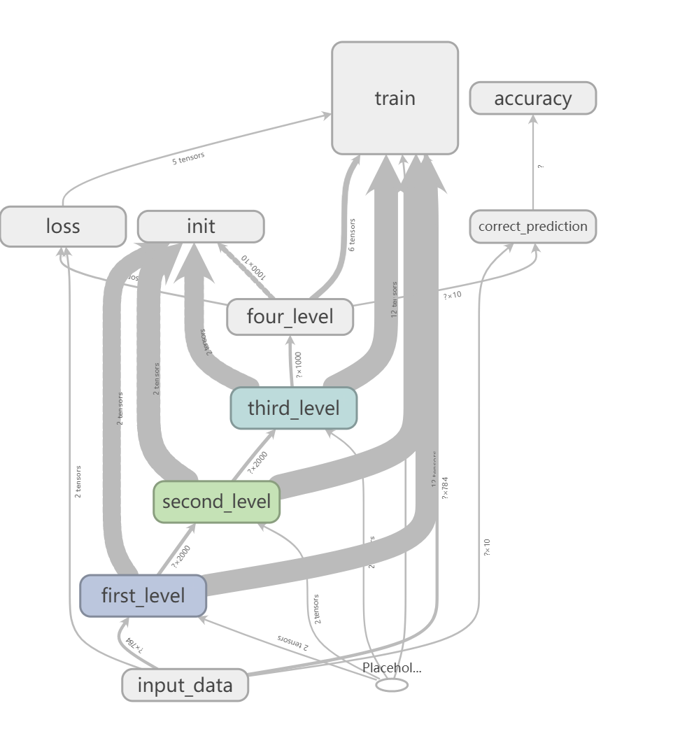
tensorboard是tensorflow的可视化面板，这种效果很像电路设计中的电路图，但又有些很不像设计图而更接近效果图（做过电路设计的可能深有感触）。

为了使效果图更好看一些，这里需要使用tensorflow.name_scope()定义一些命名空间。最后用tensorflow.summary.FileWriter("logs/",tensorflow.Session().graph)画出图像。

为了复杂一点，定义一个复杂的网络。

全部代码：

import tensorflow as tf
from tensorflow.examples.tutorials.mnist import input_data

#引入数据集
mnist = input_data.read_data_sets('MNIST_data',one_hot=True)

#设置数据集的批次
batch_size = 100
n_batch = mnist.train.num_examples // batch_size

#设置占位符
with tf.name_scope("input_data"):
    x = tf.placeholder(tf.float32,[None,784],name = "x_input")
    y = tf.placeholder(tf.float32,[None,10],name = "y_input")

#定义一个占位符，初始化keep_prob
keep_prob = tf.placeholder(tf.float32)

#创建一个稍复杂一点的神经网络
#第一层
with tf.name_scope("first_level"):
    with tf.name_scope("Weight1"):
        W1 = tf.Variable(tf.truncated_normal([784,2000],stddev=0.1))
    with tf.name_scope("Biase1"):
        B1 = tf.Variable(tf.zeros([2000]) + 0.1)
    with tf.name_scope("L1"):
        L1 = tf.nn.tanh(tf.matmul(x,W1) + B1)
        L1_drop = tf.nn.dropout(L1,keep_prob)

#第二层
with tf.name_scope("second_level"):
    with tf.name_scope("Weight2"):
        W2 = tf.Variable(tf.truncated_normal([2000,2000],stddev=0.1))
    with tf.name_scope("Biase2"):
        B2 = tf.Variable(tf.zeros([2000]) + 0.1)
    with tf.name_scope("L2"):
        L2 = tf.nn.tanh(tf.matmul(L1_drop,W2) + B2)
        L2_drop = tf.nn.dropout(L2,keep_prob)


#第三层
with tf.name_scope("third_level"):
    with tf.name_scope("Weight3"):
        W3 = tf.Variable(tf.truncated_normal([2000,1000],stddev=0.1))
    with tf.name_scope("Biase3"):
        B3 = tf.Variable(tf.zeros([1000]) + 0.1)
    with tf.name_scope("L3"):
        L3 = tf.nn.tanh(tf.matmul(L2_drop,W3) + B3)
        L3_drop = tf.nn.dropout(L3,keep_prob)

#第四层
with tf.name_scope("four_level"):
    with tf.name_scope("Weight4"):
        W4 = tf.Variable(tf.truncated_normal([1000,10],stddev=0.1))
    with tf.name_scope("Biase4"):
        B4 = tf.zeros([10]) + 0.1
    with tf.name_scope("prediction"):
        prediction = tf.nn.softmax(tf.matmul(L3_drop,W4) + B4)

#设置损失函数
with tf.name_scope("loss"):
    loss = tf.reduce_mean(tf.nn.softmax_cross_entropy_with_logits(labels = y, logits=prediction))

#设置优化器
with tf.name_scope("optimizer"):
    optimizer = tf.train.GradientDescentOptimizer(0.1)

#损失函数最小化
with tf.name_scope("train"):
    train = optimizer.minimize(loss)

#初始化变量
with tf.name_scope("init"):
    init = tf.global_variables_initializer()

#存放预测结果
with tf.name_scope("correct_prediction"):
    correct_prediction = tf.equal(tf.argmax(y,1),tf.argmax(prediction,1))

#求准确率
with tf.name_scope("accuracy"):
    accuracy = tf.reduce_mean(tf.cast(correct_prediction,tf.float32))

with tf.Session() as sess:
    sess.run(init)
    writer = tf.summary.FileWriter("logs/",sess.graph)
    for step in range(1):
        for batch in range(n_batch):
            batch_x, batch_y = mnist.train.next_batch(batch_size)
            sess.run(train,feed_dict={x:batch_x,y:batch_y,keep_prob:1.0})
        test_acc = sess.run(accuracy,feed_dict={x:mnist.test.images,y:mnist.test.labels,keep_prob:1.0})
        train_acc = sess.run(accuracy,feed_dict={x:mnist.train.images,y:mnist.train.labels,keep_prob:1.0})
        print("Iter "+ str(step) +" ,Testing Accuarcy " + str(test_acc) + " ,Training Accuarcy " + str(train_acc))

运行结果：

Iter 0 ,Testing Accuarcy 0.9398 ,Training Accuarcy 0.949164

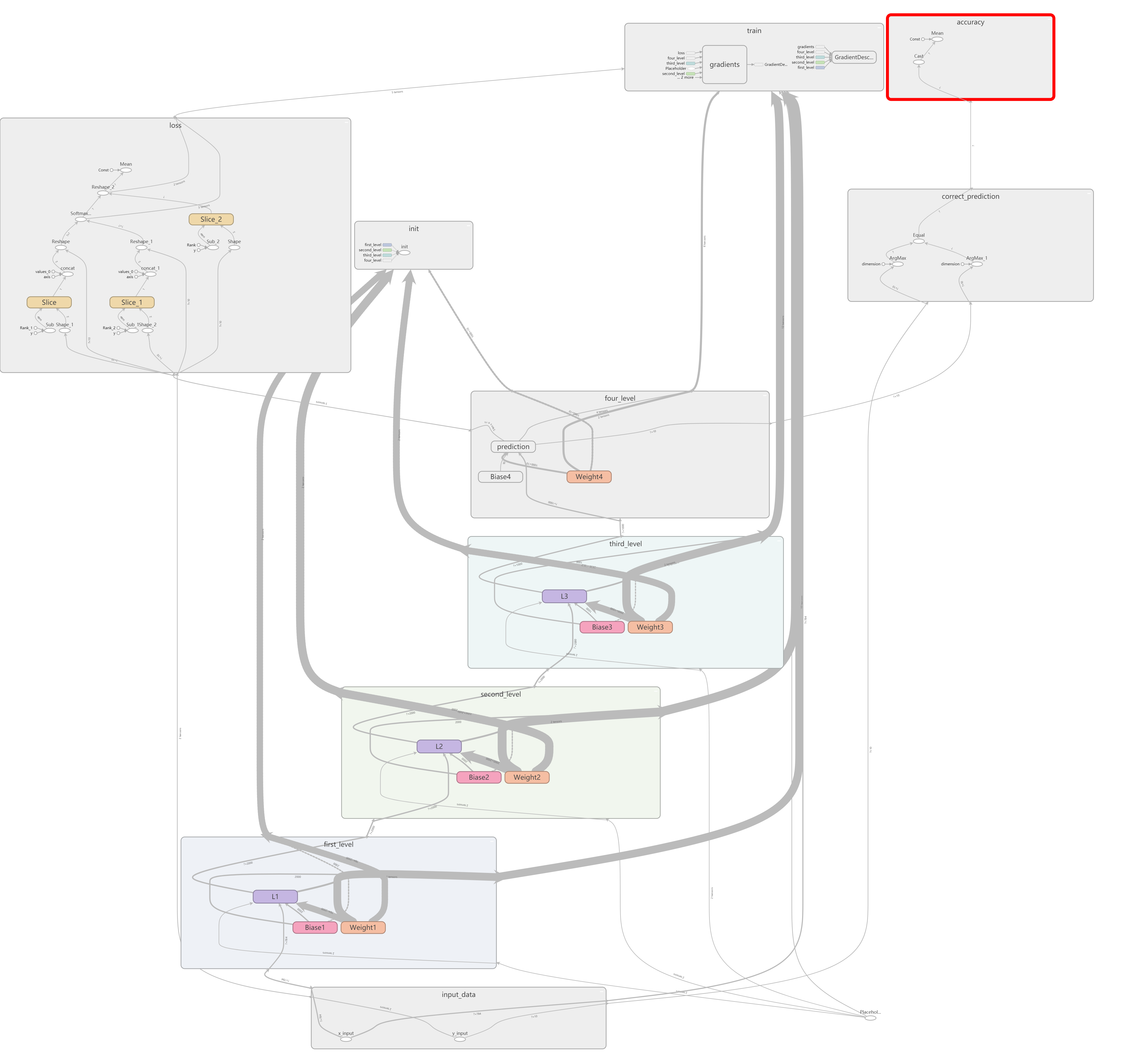
运行完毕之后，为了显示出图找到打印的log文件夹。打开命令行窗口，输入tensorboard --logdir=“log文件夹路径”，然后把生成的网址拷贝到chrome中，选择graph就可以看到图像。

如果不采用命名空间进行规划就会生成很乱的结构：（或者点开上图的节点查看）