使用 LSTM 对股票涨跌额进行预测（仅适合作业示例）

---

前言

在机器学习和深度学习中，时间序列预测是一项常见且具有挑战性的任务。LSTM（Long Short-Term Memory）是一种常用的循环神经网络（RNN）结构，善于处理序列数据与长期依赖问题。因此，许多教程会以 LSTM 为例对股票价格或涨跌进行预测。

然而，需要明确的一点是：本篇教程中的模型仅为示例用途，不具备实际预测价值。实际股市预测需要考虑极其复杂的因素，包括宏观经济、市场情绪、政策风险、突发事件等。本教程简化了许多环节，结果仅能作为参考代码与学习对象，并不建议将其用于真实的投资决策。

教程目标

使用 Pandas 读取本地股票历史数据（CSV 格式）。
使用 MinMaxScaler 对数据进行归一化。
构建简单的 LSTM 模型对股票的“收盘价”进行预测。
训练模型并可视化预测结果。
强调此模型对实际预测的局限性与滞后性，仅作为课程作业或研究演示。

数据准备

在本教程中，我们假设你已经有一份本地 CSV 文件，其中包含股票的历史交易数据。该文件应至少包含如下列：

股票代码|交易日期|开盘价|最高价|最低价|收盘价|昨收价|涨跌额|成交额(千元)
例如：000001.SZ.csv

股票代码,交易日期,开盘价,最高价,最低价,收盘价,昨收价,涨跌额,成交额(千元)
000001.SZ,2019-01-02,8.53,8.60,8.46,8.50,8.53,-0.03,1234567

请根据自己的数据进行相应调整。

代码示例

下面的代码展示了如何使用 LSTM 对股票涨跌额进行预测的基础流程。其中包含数据读取、数据预处理、模型定义与训练、以及预测结果的可视化与误差评估。

import numpy as np
import pandas as pd
import torch
from sklearn.metrics import mean_squared_error, mean_absolute_error
from sklearn.preprocessing import MinMaxScaler
from torch import nn
from torch.utils.data import DataLoader, TensorDataset
import matplotlib.pyplot as plt

# 读取本地 CSV 文件
pandas_df = pd.read_csv("000001.SZ.csv", header=0)

# 转换 '交易日期' 为 datetime 类型并按日期排序
pandas_df['交易日期'] = pd.to_datetime(pandas_df['交易日期'], errors='coerce')
pandas_df.sort_values('交易日期', inplace=True)

# 去除空值行
pandas_df = pandas_df.dropna()

# 选择用于训练的特征列
features = ['开盘价', '最高价', '最低价', '收盘价', '昨收价', '涨跌额', '成交额(千元)']
data = pandas_df[features]

# 使用 MinMaxScaler 对特征进行归一化
scaler = MinMaxScaler()
scaled_data = scaler.fit_transform(data)
scaled_df = pd.DataFrame(scaled_data, columns=features, index=pandas_df['交易日期'])

# 将数据按时间分割
train_data = scaled_df[scaled_df.index < '2020-01-01']
test_data = scaled_df[scaled_df.index >= '2020-01-01']

# 创建时间序列数据集的函数，使用过去 N 天的数据来预测未来的收盘价
def create_dataset_for_profit(df, _time_step=60):
    X, y = [], []
    for i in range(len(df) - _time_step - 1):
        X.append(df.iloc[i:(i + _time_step)].values)  # 特征
        y.append(df.iloc[i + _time_step, 3])  # 预测目标，选择收盘价（"收盘价"的索引是 3）
    return np.array(X), np.array(y)

# 创建时间序列数据集
time_step = 20  # 使用过去 60 天的数据来预测未来一天的收盘价

# 创建训练集和测试集的数据集
X_train, y_train = create_dataset_for_profit(train_data, time_step)
X_test, y_test = create_dataset_for_profit(test_data, time_step)

# 检查训练集和测试集的形状
print(X_train.shape, y_train.shape)
print(X_test.shape, y_test.shape)


# 将数据转换为 PyTorch 张量
X_train_tensor = torch.tensor(X_train, dtype=torch.float32)
y_train_tensor = torch.tensor(y_train, dtype=torch.float32).view(-1, 1)
X_test_tensor = torch.tensor(X_test, dtype=torch.float32)
y_test_tensor = torch.tensor(y_test, dtype=torch.float32).view(-1, 1)

# 创建训练集和测试集的 DataLoader
train_data = TensorDataset(X_train_tensor, y_train_tensor)
test_data = TensorDataset(X_test_tensor, y_test_tensor)

train_loader = DataLoader(train_data, batch_size=32, shuffle=False)
test_loader = DataLoader(test_data, batch_size=32, shuffle=False)


class LSTMModel(nn.Module):
    def __init__(self, input_size, hidden_layer_size, output_size):
        super(LSTMModel, self).__init__()

        # 第一层 LSTM
        self.lstm1 = nn.LSTM(input_size, hidden_layer_size, batch_first=True)

        # 第二层 LSTM
        self.lstm2 = nn.LSTM(hidden_layer_size, hidden_layer_size, batch_first=True)

        # 全连接层
        self.fc = nn.Linear(hidden_layer_size, output_size)

    def forward(self, x):
        # 第一层 LSTM
        out, (hn, cn) = self.lstm1(x)

        # 第二层 LSTM
        out, (hn, cn) = self.lstm2(out)

        # 只取最后一时刻的输出
        out = self.fc(out[:, -1, :])
        return out

# 模型超参数
input_size = len(features)  # 特征数量
hidden_layer_size = 32  # 隐藏层神经元个数
output_size = 1  # 预测收盘价

# 初始化模型
model = LSTMModel(input_size=input_size, hidden_layer_size=hidden_layer_size, output_size=output_size)

# 打印模型结构
print(model)

# 定义损失函数和优化器
criterion = nn.MSELoss()  # 由于目标是预测连续数值（收盘价），我们使用 MSELoss
optimizer = torch.optim.Adam(model.parameters(), lr=0.001)

# 训练模型
epochs = 100
for epoch in range(epochs):
    model.train()
    running_loss = 0.0
    for inputs, labels in train_loader:
        # 清零梯度
        optimizer.zero_grad()

        # 前向传播
        outputs = model(inputs)

        # 计算损失
        loss = criterion(outputs, labels)

        # 反向传播
        loss.backward()

        # 更新参数
        optimizer.step()

        # 累积损失
        running_loss += loss.item()

    # 每 5 个 epoch 输出一次损失
    if (epoch + 1) % 5 == 0:
        print(f'Epoch [{epoch + 1}/{epochs}], Loss: {running_loss / len(train_loader)}')


# 测试模型
model.eval()
predictions = []
real_values = []

with torch.no_grad():
    for inputs, labels in test_loader:
        outputs = model(inputs)
        predictions.append(outputs.numpy())
        real_values.append(labels.numpy())

# 将预测结果转换为 numpy 数组
predictions = np.concatenate(predictions)
real_values = np.concatenate(real_values)

# 可视化预测结果


# 创建图形，设置图形大小
plt.figure(figsize=(12, 6))

# 绘制真实值和预测值
plt.plot(real_values, color='blue', label='真正的收盘价', linewidth=2, linestyle='-', marker='o', markersize=6, alpha=0.8)
plt.plot(predictions, color='red', label='预测的收盘价', linewidth=2, linestyle='--', marker='x', markersize=6, alpha=0.8)

# 添加标题
plt.title('股票收盘价预测 (LSTM)', fontsize=16, fontweight='bold')

# 设置 x 和 y 轴的标签
plt.xlabel('时间', fontsize=14)
plt.ylabel('收盘价 ', fontsize=14)

# 添加网格，设置透明度
plt.grid(True, which='both', linestyle='--', linewidth=0.5, alpha=0.6)

# 设置 x 轴为时间格式
plt.xticks(rotation=45, fontsize=12)
plt.yticks(fontsize=12)

# 添加图例
plt.legend(fontsize=12)

# 显示图表
plt.tight_layout()  # 自动调整布局
plt.show()

# 计算均方误差（MSE）
mse = mean_squared_error(real_values, predictions)
print(f'Mean Squared Error (MSE): {mse}')

# 计算均方根误差（RMSE）
rmse = np.sqrt(mse)
print(f'Root Mean Squared Error (RMSE): {rmse}')

# 计算平均绝对误差（MAE）
from sklearn.metrics import mean_absolute_error
mae = mean_absolute_error(real_values, predictions)
print(f'Mean Absolute Error (MAE): {mae}')

结果展示

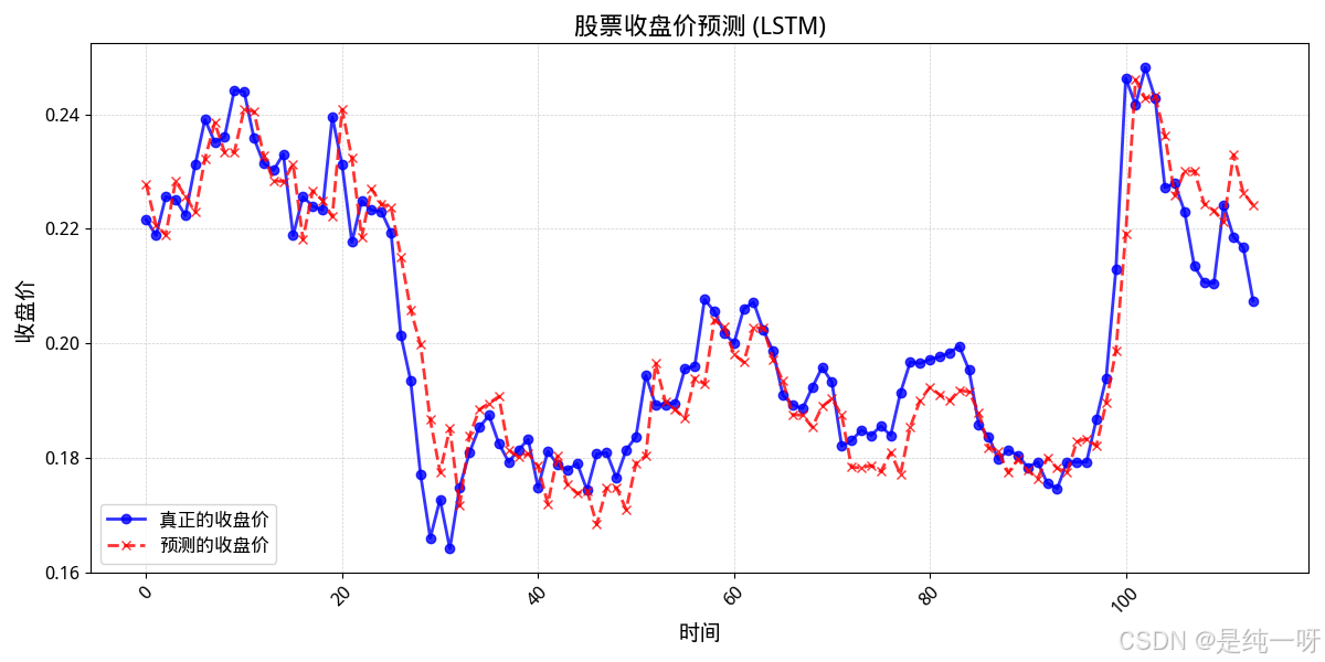
Mean Squared Error (MSE): 6.731566827511415e-05
Root Mean Squared Error (RMSE): 0.008204612880945206
Mean Absolute Error (MAE): 0.006247698795050383

从图像可以看出：
股票价格变化复杂且多变，仅使用过去的价格数据难以捕捉未来的行情变动。模型在实际使用中通常会表现出滞后性与不稳定性，预测结果往往与现实走势有较大偏差。