Andrew Ng Machine Learning——Work(Four)——Feedback neural network(Based on Python 3.7)

                   Python 3.7

所用数据集链接：反向传播网络所用数据集(ex4data1.mat,ex4weights.mat),提取码：c3yy

Feedback neural network

题目：仍然是手写数字识别，不过本次要求从头开始完整地训练一个神经网络，并且在其中采用反向传播算法减小误差。数据集中的X为（5000，400）的矩阵，即有5000个样本，每个样本选取了400个像素点。y为（5000，1）,指明每一个样本类别。

首先导入用到的包：

1.0 Package

import numpy as np
# 数据处理
import matplotlib.pyplot as plt
# 绘图
from scipy.io import loadmat
# 加载矩阵文件
from sklearn.metrics import classification_report
# 分类报告
import scipy.optimize as opt
# 高级优化函数

1.1 Load data

然后读入数据：

def load_data(path):
# 定义函数，传入路径
    data=loadmat(path)
# 读取矩阵文件
    raw_x=data['X']
    raw_y=data['y'].flatten()
# 根据索引读取x,y并将y展开（方便后续与模型预测出的y_pred比较）
    return raw_x,raw_y
# 返回
raw_x,raw_y=load_data('ex4data1.mat')
#print(np.unique(raw_y))
# 查看raw_y中一共有几类数据，也就是看分为几类，从而确定输出层激活单元数
# raw_x为（5000，400），raw_y为（5000，)

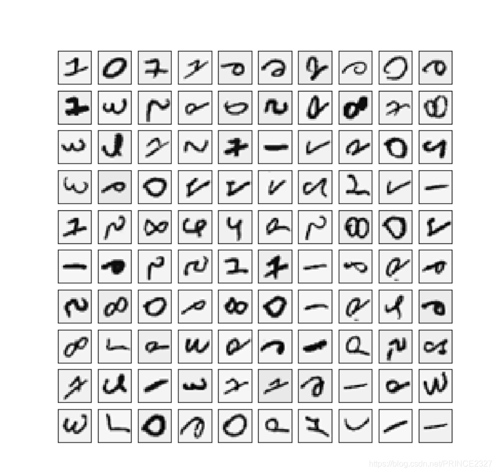
1.2 Visualization data

下面进行数据的可视化，选取100个样本进行可视化：

def view_data():
# 定义函数
    data_index=np.random.randint(0,5000,100)
# 在样本中随机选取100个
    data_sample=raw_x[data_index]
# 找到对应样本
    fig,ax=plt.subplots(10,10,sharex=True,sharey=True,figsize=(8,8))
# 创建画布和对象，其中前两个参数是指对象在画布上的分布，也即10行10列
# 注意此时的ax是一个数组
    for i in range(10):
        for j in range(10):            ax[i,j].matshow(data_sample[10*i+j].reshape(20,20),cmap='gray_r')
# 绘制矩阵，记得把样本reshape成（20，20）的
    plt.xticks([])
    plt.yticks([])
# 去掉坐标轴
    plt.show()
# 可视化
view_data()

结果如下：

1.3 Data preprocess

下面进行数据预处理：

def data_preprocess(raw_x,raw_y):
# 定义函数，传入参数
    x=np.insert(raw_x,0,1,axis=1)
# 加一列1，向量化
    y=[]
    for i in raw_y:
        y_array=np.zeros(10)
        y_array[i-1]=1
        y.append(y_array)
# 将y转换为独热编码
    return x,np.array(y)
# 返回处理后的x,y（记得把y的类型设置成数组）
x,y=data_preprocess(raw_x,raw_y)
print(x.shape,y.shape)
# 查看形状 （5000，401），（5000，10）

1.4 Load weights

加载给定的权重（只是为了看看形状，后续还是需要我们自己训练网络权重）：

def load_weight(path):
# 定义函数，传入参数
    data=loadmat(path)
# 读取矩阵文件
    theta1=data['Theta1']
    theta2=data['Theta2']
# 根据索引值区分theta1和theta2
    return theta1,theta2
theta1,theta2=load_weight('ex4weights.mat')
print(theta1.shape,theta2.shape)
# 查看形状 (25,401),(10,26)

1.5 Unrolling data

下面定义序列化函数，可以用来展开数组：

def unrolling(theta1,theta2):
# 定义函数，传入参数
    theta=np.r_[theta1.flatten(),theta2.flatten()]
# 将theta1,theta2展开再合并
    return theta
theta=unrolling(theta1,theta2) 
print(theta.shape)
# (10285,)

1.6 Deserialize data

展开是为了在优化函数中传入向量，但其它地方我们也需要矩阵形式的参数，故再定义解序列化函数：

def deserialize(theta):
# 定义函数，传入从参数
    theta1=theta[:25*401].reshape(25,401)
# 取前25*401个数恢复成25*401的数组（二维数组）
    theta2=theta[25*401:].reshape(10,26)
# 同上
    return theta1,theta2
theta1,theta2=deserialize(theta)

1.7 Sigmoid function

定义激活函数：

def sigmoid(z):
    return 1/(1+np.exp(-z))

1.8 Sigmoid diff

定义激活函数倒数，后续在反向传播时候会用到：

def sigmoid_gradient(z):
    return sigmoid(z)*(1-sigmoid(z))
# 导数与原函数的关系读者可自行推导

1.9 Feedforward propagation

开始前向传播：

def feedforward(theta,x):
    theta1,theta2=deserialize(theta)
    a1=x
    z2=a1@theta1.T
    a2=np.insert(sigmoid(z2),0,1,axis=1)
    z3=a2@theta2.T
    h=sigmoid(z3)
    return a1,z2,a2,z3,h
# 具体公式见上图

1.10 Costfunction

定义代价函数：

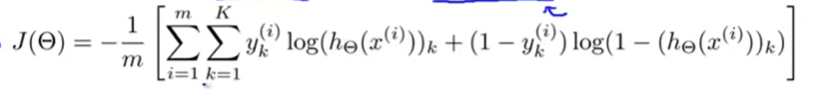
def costfunction(theta,x,y):
# 定义函数
    a1,z2,a2,z3,h=feedforward(theta,x)
# 导入前向传播的参数
    cost=-y*np.log(h)-(1-y)*np.log(1-h)
    return cost.sum()/len(x)
# 计算代价函数
cost=costfunction(theta,x,y)
#print(cost) #读取的权重对应的值为0.28多

1.11 Regularized costfunction

下面对于代价函数进行正则化：

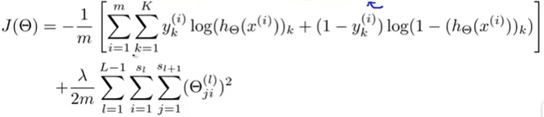
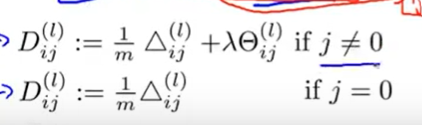
def regularized_costfunction(theta,x,y,l):
    theta1,theta2=deserialize(theta)
    reg=np.sum(theta1[:,1:]**2)+np.sum(theta2[:,1:]**2)
    return reg*l/(2*len(x))+costfunction(theta,x,y)
re_cost=regularized_costfunction(theta,x,y,1)
# 都是数学公式，很简单
#print(re_cost) #读取的权重对应的值大约为0.38多

1.12 Gradient function

下面定义梯度函数：

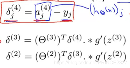
def gradient(theta,x,y):
    theta1,theta2=deserialize(theta)
    a1,z2,a2,z3,h=feedforward(theta,x)
    d3=h-y
    d2=d3@theta2[:,1:]*sigmoid_gradient(z2)
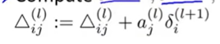
    D2=d3.T@a2
    D1=d2.T@a1
    D=(1/len(x))*unrolling(D1,D2)
 # 计算公式可自行推导，一点微积分就够了。返回的D是展开后的全局梯度
    return D

1.13 Regularized gradient

将梯度正则化：

def regularized_gradient(theta,x,y,l):
    theta1,theta2=deserialize(theta)
    a1,z2,a2,z3,h=feedforward(theta,x)
    D1,D2=deserialize(gradient(theta,x,y))
    theta1[:,0]=0
    theta2[:,0]=0
# 不对theta0正则化
    reg_D1=D1+(l/len(x))*theta1
    reg_D2=D2+(l/len(x))*theta2
    return unrolling(reg_D1,reg_D2)
# 返回正则化后的梯度（展开为一维数组）

1.14 Gradient check

梯度检验，确保梯度函数正确：

def gradient_checking(theta, x, y, e):
    def grad(plus, minus):
        return (regularized_costfunction(plus, x, y,1) - regularized_costfunction(minus, x, y,1)) / (e * 2)
# 返回粗略计算的梯度
   
    grad = [] 
    for i in range(len(theta)):
        plus = theta.copy() 
        minus = theta.copy()
        plus[i] = plus[i] + e
        minus[i] = minus[i] - e
        grad_i = grad(plus, minus)
       ngrad.append(grad_i)
    
    grad = np.array(grad)
# 转换为数组
    analytic_grad = regularized_gradient(theta, x, y,1)
# 返回梯度函数计算的梯度
    diff = np.linalg.norm(grad - analytic_grad) / np.linalg.norm(grad + analytic_grad)
# 看看两者差别，最多差几位小数

    print('nRelative Difference: {}'.format(diff))
gradient_checking(theta, x, y, 0.0001)

顺便说一下，正式跑网络时候梯度检测一定要关掉。

1.15 Random initial

def random_init(size):
    return np.random.uniform(-0.1,0.1,size)
# 在-0.1到0.1区间中返回size个数构成一个数组

1.16 Training model

下面开始训练模型：

def training(x, y):
    acc=[]
    for i in range（200):
        init_theta = random_init(10285)  # 25*401 + 10*26
        res = opt.minimize(fun=regularized_costfunction,
                           x0=init_theta,
                           args=(x, y, 1),
                           method='TNC',
                           jac=regularized_gradient,
                           options={'maxiter': i})
        _, _, _, _, h = feedforward(res.x,x)
        y_pred = np.argmax(h, axis=1) + 1
        a=np.mean(y_pred==raw_y)
        acc.append(a)
    fig,ax=plt.subplots(figsize=(6,6))
    ax.plot(np.arange(200),acc)
    plt.ylim(0,1.0)
    ax.set_xlabel('Iterations')
    ax.set_ylabel('Accuracy')
    ax.set_title('Iterations VS Accuracy')
    plt.show()    
    return res
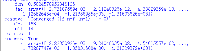
result=training(x,y)
print(result)
# 这一部分添加了准确率随迭代次数的关系图，所以运行起来相对比较慢，读者可以去掉画图部分。

输出如下：

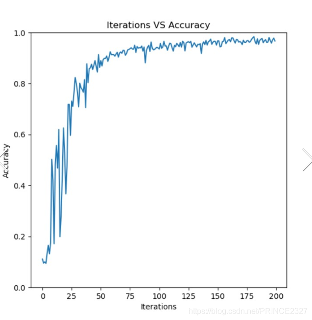
看到前期振荡比较剧烈，到后期会好很多。

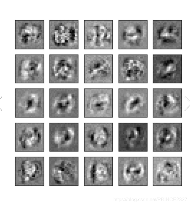
1.17 Visualization hidden layer

下面可视化隐层：

def visualization_hidden(theta):
    theta1,theta2 = deserialize(theta)
    theta1 = theta1[:, 1:]
    fig,ax_array = plt.subplots(5, 5, sharex=True, sharey=True, figsize=(6,6))
    for i in range(5):
        for j in range(5):
            ax_array[i, j].matshow(theta1[r * 5 + c].reshape(20, 20), cmap='gray_r')
            plt.xticks([])
            plt.yticks([])
    plt.show()
visualization_hidden(result.x)
# 传入的是我们训练好的theta

结果如下：

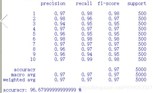
1.18 Evalute model

下面评估模型：

def accuracy(result, x, y):
    _, _, _, _, h = feedforward(result.x,x)
    y_pred = np.argmax(h, axis=1) + 1
    acc=np.mean(y_pred==y)
    print(classification_report(y, y_pred))
# 分别传入真实标签与预测标签
    print('accuracy:',np.mean(acc)*100,'%')
accuracy(result,x,raw_y)

结果如下：

1.19 Apply model

应用这个模型只需要写一段程序，可以将手写体图片转换为20*20的灰度图像即可。

1.20 All

下面给出完整代码：

import numpy as np
import matplotlib.pyplot as plt
from scipy.io import loadmat
from sklearn.metrics import classification_report
import scipy.optimize as opt
def load_data(path):
    data=loadmat(path)
    raw_x=data['X']
    raw_y=data['y'].flatten()
    return raw_x,raw_y
raw_x,raw_y=load_data('ex4data1.mat')
print(raw_y.shape)
def view_data():
    data_index=np.random.randint(0,5000,100)
    data_sample=raw_x[data_index]
    fig,ax=plt.subplots(10,10,sharex=True,sharey=True,figsize=(8,8))
    for i in range(10):
        for j in range(10):
            ax[i,j].matshow(data_sample[10*i+j].reshape(20,20),cmap='gray_r')
    plt.xticks([])
    plt.yticks([])
    plt.show()
view_data()
def data_preprocess(raw_x,raw_y):
    x=np.insert(raw_x,0,1,axis=1)
    y=[]
    for i in raw_y:
        y_array=np.zeros(10)
        y_array[i-1]=1
        y.append(y_array)
    return x,np.array(y)
x,y=data_preprocess(raw_x,raw_y)
print(x.shape,y.shape)

def load_weight(path):
    data=loadmat(path)
    theta1=data['Theta1']
    theta2=data['Theta2']
    return theta1,theta2
theta1,theta2=load_weight('ex4weights.mat')
print(theta1.shape,theta2.shape)

def unrolling(theta1,theta2):
    theta=np.r_[theta1.flatten(),theta2.flatten()]
    return theta
theta=unrolling(theta1,theta2)
print(theta.shape)

def deserialize(theta):
    theta1=theta[:25*401].reshape(25,401)
    theta2=theta[25*401:].reshape(10,26)
    return theta1,theta2
theta1,theta2=deserialize(theta)

def sigmoid(z):
    return 1/(1+np.exp(-z))

def sigmoid_gradient(z):
    return sigmoid(z)*(1-sigmoid(z))

def feedforward(theta,x):
    theta1,theta2=deserialize(theta)
    a1=x
    z2=a1@theta1.T
    a2=np.insert(sigmoid(z2),0,1,axis=1)
    z3=a2@theta2.T
    h=sigmoid(z3)
    return a1,z2,a2,z3,h
def costfunction(theta,x,y):
    a1,z2,a2,z3,h=feedforward(theta,x)
    cost=-y*np.log(h)-(1-y)*np.log(1-h)
    return cost.sum()/len(x)
cost=costfunction(theta,x,y)
#print(cost)

def regularized_costfunction(theta,x,y,l):
    theta1,theta2=deserialize(theta)
    reg=np.sum(theta1[:,1:]**2)+np.sum(theta2[:,1:]**2)
    return reg*l/(2*len(x))+costfunction(theta,x,y)
re_cost=regularized_costfunction(theta,x,y,1)
#print(re_cost)

def random_init(size):
    return np.random.uniform(-0.12,0.12,size)

def gradient(theta,x,y):
    theta1,theta2=deserialize(theta)
    a1,z2,a2,z3,h=feedforward(theta,x)
    d3=h-y
    d2=d3@theta2[:,1:]*sigmoid_gradient(z2)
    D2=d3.T@a2
    D1=d2.T@a1
    D=(1/len(x))*unrolling(D1,D2)
    return D
def regularized_gradient(theta,x,y,l):
 #   theta1,theta2=deserialize(theta)
    a1,z2,a2,z3,h=feedforward(theta,x)
    D1,D2=deserialize(gradient(theta,x,y))
    theta1[:,0]=0
    theta2[:,0]=0
    reg_D1=D1+(l/len(x))*theta1
    reg_D2=D2+(l/len(x))*theta2
    return unrolling(reg_D1,reg_D2)
def gradient_checking(theta, x, y, e):
    def grad(plus, minus):
        return (regularized_costfunction(plus, x, y,1) - regularized_costfunction(minus, x, y,1)) / (e * 2)
# 返回粗略计算的梯度
   
    grad = [] 
    for i in range(len(theta)):
        plus = theta.copy() 
        minus = theta.copy()
        plus[i] = plus[i] + e
        minus[i] = minus[i] - e
        grad_i = grad(plus, minus)
       ngrad.append(grad_i)
    
    grad = np.array(grad)
# 转换为数组
    analytic_grad = regularized_gradient(theta, x, y,1)
# 返回梯度函数计算的梯度
    diff = np.linalg.norm(grad - analytic_grad) / np.linalg.norm(grad + analytic_grad)
# 看看两者差别，最多差几位小数

    print('nRelative Difference: {}'.format(diff))
gradient_checking(theta, x, y, 0.0001)


def training(x, y):
    acc=[]
    for i in range(20):
        init_theta = random_init(10285)  # 25*401 + 10*26
        res = opt.minimize(fun=regularized_costfunction,
                           x0=init_theta,
                           args=(x, y, 1),
                           method='TNC',
                           jac=regularized_gradient,
                           options={'maxiter': i})
        _, _, _, _, h = feedforward(res.x,x)
        y_pred = np.argmax(h, axis=1) + 1
        a=np.mean(y_pred==raw_y)
        acc.append(a)
    fig,ax=plt.subplots(figsize=(6,6))
    ax.plot(np.arange(20),acc)
    plt.ylim(0,1.0)
    ax.set_xlabel('Iterations')
    ax.set_ylabel('Accuracy')
    ax.set_title('Iterations VS Accuracy')
    plt.show()    
    return res
result=training(x,y)
print(result)
    
def accuracy(result, x, y):
    _, _, _, _, h = feedforward(result.x,x)
    y_pred = np.argmax(h, axis=1) + 1
    acc=np.mean(y_pred==y)
    print(classification_report(y, y_pred))
    print('accuracy:',np.mean(acc)*100,'%')
accuracy(result,x,raw_y)
def visualization_hidden(theta):
    theta1,theta2 = deserialize(theta)
    theta1 = theta1[:, 1:]
    fig,ax_array = plt.subplots(5, 5, sharex=True, sharey=True, figsize=(6,6))
    for i in range(5):
        for j in range(5):
            ax_array[i, j].matshow(theta1[r * 5 + c].reshape(20, 20), cmap='gray_r')
            plt.xticks([])
            plt.yticks([])
    plt.show()
visualization_hidden(result.x)
# 传入的是我们训练好的theta

多加练习。

未经允许，请勿转载。

欢迎交流。