


详解谷歌机器翻译模型:Transformer
- 1. 模型框/架
- 2. 具体的步骤
- 2.1 Embedding algorithm
- 2.2 使用单词进行具体说明
- 2.3 三个向量 Q u e r y v e c t o r , K e y v e c t o r 和 V a l u e v e c t o r Query\,vector,Key\,vector和Value\, vector Queryvector,Keyvector和Valuevector的细节
- 2.4 向量化表示,三个向量的矩阵话运算表示
- 2.5 Multi-Headed
- 2.6 位置编码 Positional Encoding
- 2.7 残差块
- 2.8 解码器工作
- 2.9 最后的Linear 和Softmax Layer
- 3. 训练的一些细节
- 4.参考资料
1. 模型框/架
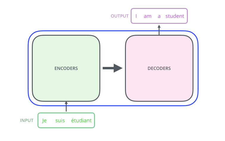
Transformer 是谷歌提出的机器翻译模型。其包括了一个编码器Encoder和Decoder,这是一个翻译的模型,将源语言input进编码器,然后通过解码器输出模型 。可以表示为如下
输入编码器是一系列的编码器的集合,这个编码器是,论文中包括了六个编码器(六个并没有特殊的要求),同样,解码器就是也是由六个编码器堆叠而成的如图2。
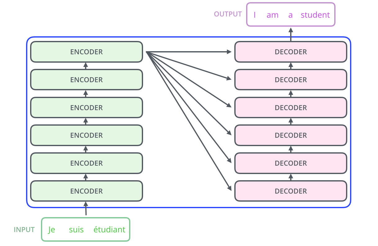
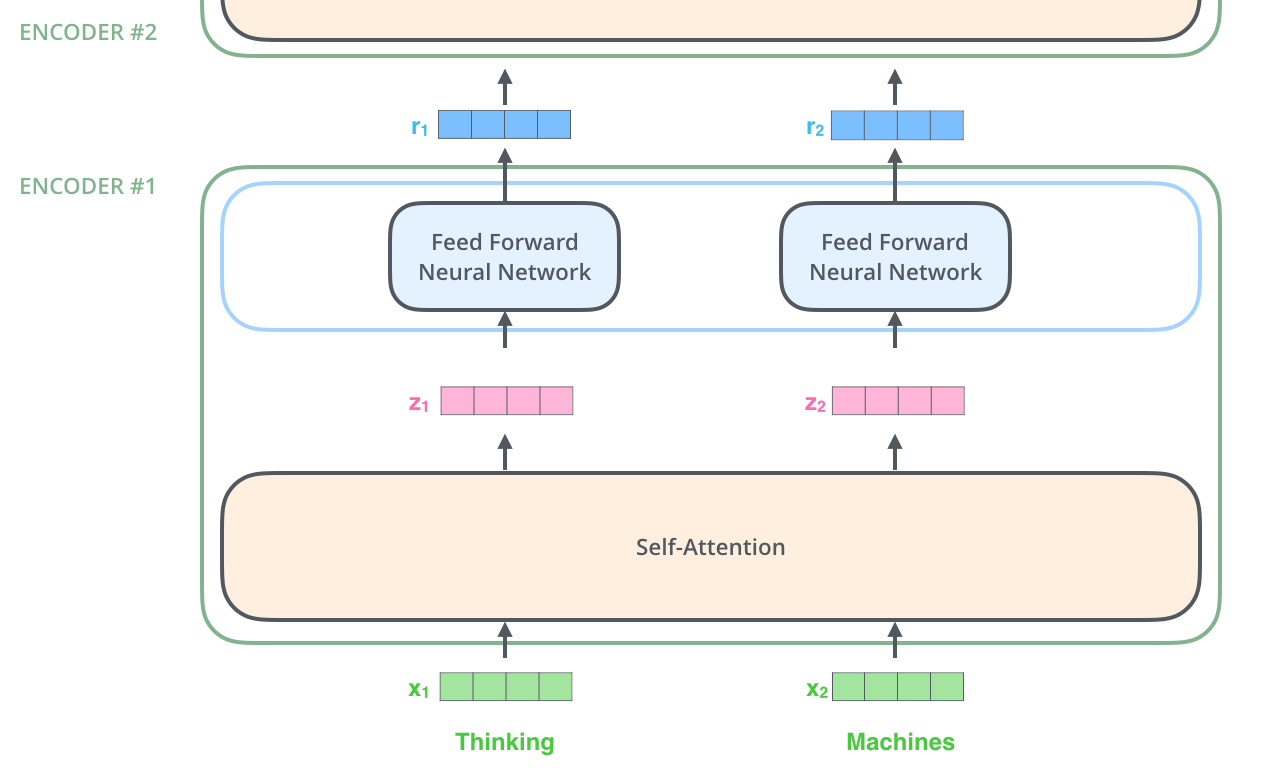
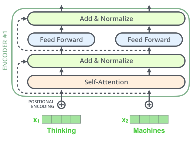
六个编码器都是一样的结构(尽管他们并不共享权重),每一个都可以分解为如下的两个子层,即子注意力。
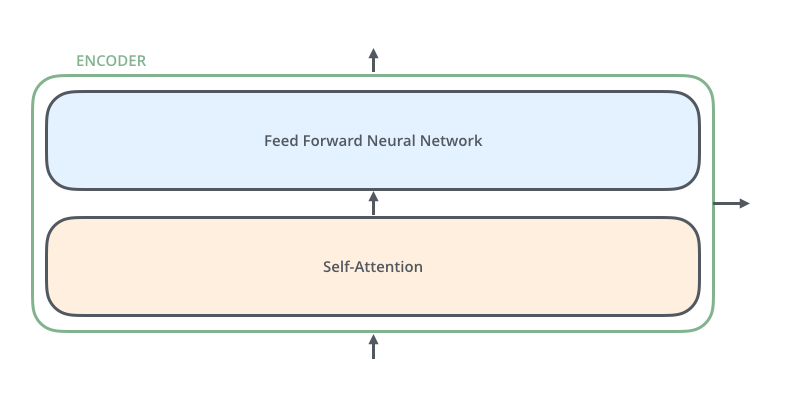
输入首先经过一个Self-Attention层作为输入,这一层在编码一个句子中指定的单词的时候可以帮助观察到其他的单词,输出。
Self-Attention的输出被送入前馈神经网络,并且一个句子的每个单词在送入前馈神经网络中都是独立的,不会交叉输入。
解码器也有这些层,但是在自注意层和前馈层还有一个Encoder-Decoder Attention 层,并且在堆叠的这些编码器的顶部通往每一个,堆叠的解码器中的每一个Encoder-Decoder Attention 层。

2. 具体的步骤
2.1 Embedding algorithm
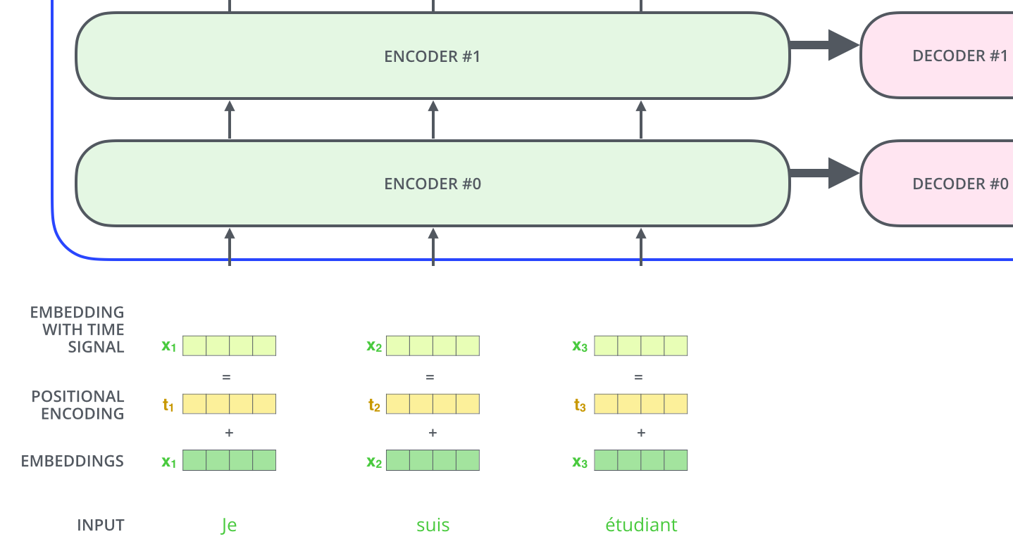
一般都会把每一个单词使用embedding algorithm编码成一个向量,这种编码发生在编码器最底部的输入之前。如下是把其编码成了512个维度:
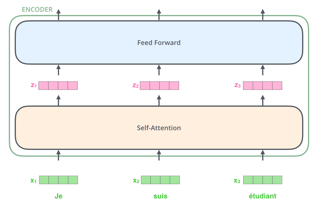
在上图我们可以看到一个句子的输入会在自己对应的位置开始输入,一般会设置一个输入的最长的长度如N=1000即每次最多能输入和翻译1000个单词。
2.2 使用单词进行具体说明
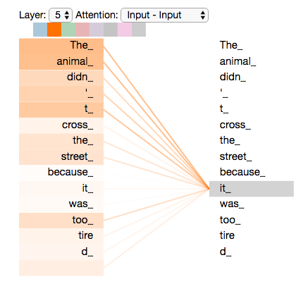
对于下面这句话:
The animal didn’t cross the street because it was too tired. 中的 it 指的是什么,自注意力就可以把它和 animal 相关联。
2.3 三个向量 Q u e r y v e c t o r , K e y v e c t o r 和 V a l u e v e c t o r Query\,vector,Key\,vector和Value\, vector Queryvector,Keyvector和Valuevector的细节
step 1 后面的计算position都以 1 1 1为标准
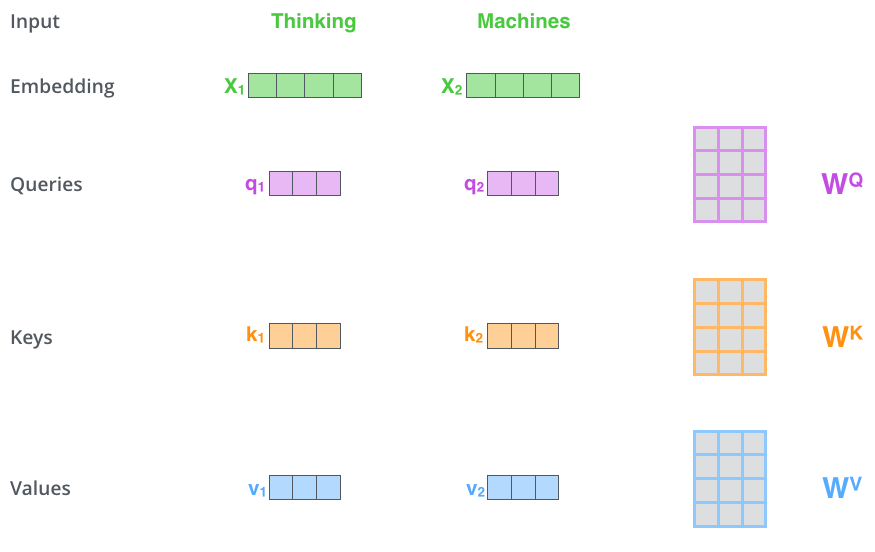
第一步是根据每一个输入的向量中计算出三个向量: Q u e r y v e c t o r , K e y v e c t o r 和 V a l u e v e c t o r Query\,vector,Key\,vector和Value\, vector Queryvector,Keyvector和Valuevector, 这些向量通过原始输入乘法上三个矩阵(在训练中学习到的)生成。注意到这些新的 v e c t o r vector vector的维度要比原始的输入的维度小很多,只有64(假设)。
step 2
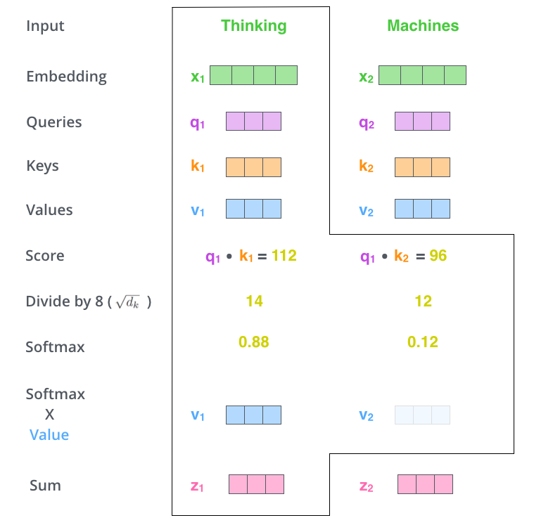
第二步是计算一个 s c o r e score score ,按照比如第一个单词 x 1 x_1 x1: s c o r e ( x 1 , x 1 ) = q 1 ⋅ k 1 , s c o r e ( x 1 , x 2 ) = q 1 , k 2 ⋯ score(x_1,x_1) = q1\cdot k1,score(x_1,x_2)=q1,k2 \cdots score(x1,x1)=q1⋅k1,score(x1,x2)=q1,k2⋯
step3
把这些 s c o r e / 8 ( 让 其 为 K e y v e c t o r 的 维 度 ) score/8(让其为\sqrt{Key\,vector的维度}) score/8(让其为Keyvector的维度),从而获得更为稳定的梯度。然后使用Softmax进行概率的计算。来得到每一个单词的在这个位置(position)的占比或重要程度。
接着把每一个 ( V a l u e v e c t o r ) ∗ ( S o f t m a x s c o r e ) (Value \,vector)*(Softmax\,score) (Valuevector)∗(Softmaxscore)进行加权求和(权重为 S o f t m a x s c o r e Softmax\,score Softmaxscore),来得到这一位置的最后输出向量 z 1 z_1 z1。
2.4 向量化表示,三个向量的矩阵话运算表示
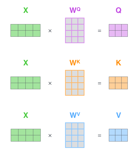
可以从上图看出,输入的横向量堆砌而成的矩阵,经过和三个变换矩阵的乘积然后得到
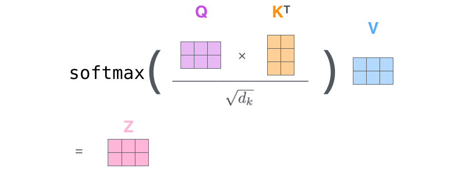
Q u e r y m a t r i x , K e y m a t r i x 和 V a l u e m a t r i x Query\,matrix,Key\,matrix和Value\, matrix Querymatrix,Keymatrix和Valuematrix这三个矩阵,然后经过一系列运算得到最终的 Z m a t r i x Z matrix Zmatrix
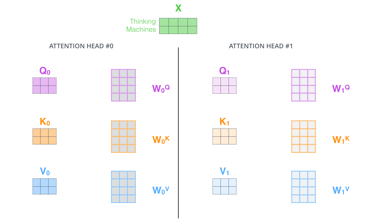
2.5 Multi-Headed
我们希望能够生成多组 Q , K , V Q,K,V Q,K,V从而更好的提升模型的表达效果
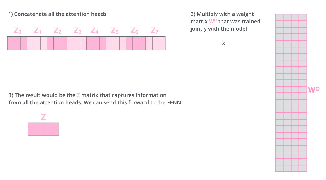
对于生成的各组z我们也会通过增广矩阵的形式并乘上一个权重矩阵从而得到最后的 z z z ,如下图所示
2.6 位置编码 Positional Encoding
这里方法用到的理念:把这些只跟位置相关的值加入到 e m b e d d i n g embedding embedding后,把他们投影到 Q / K / V Q/K/V Q/K/V后就可以在 d o t p r o d u c t a t t e n t i o n dot\,product\,attention dotproductattention过程中提供有效的距离。
原文提出了两种方式:一种是训练出一个位置编码,第二种是用原文使用的三角函数编码的方式,其具体公式如下:
P
E
(
p
o
s
)
=
{
s
i
n
(
p
o
s
1000
0
i
d
m
o
d
e
l
)
i
f
i
为
偶
数
c
o
s
(
p
o
s
1000
0
i
−
1
d
m
o
d
e
l
)
i
f
i
为
奇
数
注
:
使
用
三
角
函
数
是
因
为
三
角
函
数
的
性
质
既
可
以
考
虑
到
绝
对
位
置
又
可
以
考
虑
到
相
对
位
置
c
o
s
(
α
+
β
)
=
c
o
s
(
α
)
∗
c
o
s
(
β
)
−
s
i
n
(
α
)
∗
s
i
n
(
β
)
s
i
n
(
α
+
β
)
=
s
i
n
(
α
)
∗
c
o
s
(
β
)
+
c
o
s
(
α
)
∗
s
i
n
(
β
)
通
过
这
些
公
式
可
以
通
过
位
置
k
的
先
行
表
达
来
表
示
位
置
k
+
x
PE(pos)= \begin{cases} sin\left( \cfrac {pos}{10000^{\cfrac{i}{d_{model}}}}\right) if\, i为偶数 \\ cos\left( \cfrac {pos}{10000^{\cfrac{i-1}{d_{model}}}}\right) if\,i为奇数 \end{cases}\\ 注:使用三角函数是因为三角函数的性质既可以考虑到绝对位置又可以考虑到相对位置\\ cos(\alpha + \beta)=cos(\alpha)*cos(\beta)-sin(\alpha)*sin(\beta)\\ sin(\alpha+\beta)=sin(\alpha)*cos(\beta)+cos(\alpha)*sin(\beta)\\ 通过这些公式可以通过位置k的先行表达来表示位置k+x
PE(pos)=⎩⎪⎪⎪⎪⎪⎪⎪⎪⎪⎪⎪⎪⎨⎪⎪⎪⎪⎪⎪⎪⎪⎪⎪⎪⎪⎧sin⎝⎜⎜⎜⎛10000dmodelipos⎠⎟⎟⎟⎞ifi为偶数cos⎝⎜⎜⎜⎛10000dmodeli−1pos⎠⎟⎟⎟⎞ifi为奇数注:使用三角函数是因为三角函数的性质既可以考虑到绝对位置又可以考虑到相对位置cos(α+β)=cos(α)∗cos(β)−sin(α)∗sin(β)sin(α+β)=sin(α)∗cos(β)+cos(α)∗sin(β)通过这些公式可以通过位置k的先行表达来表示位置k+x
# 具体的编码代码实现,可以了解一下
class PositionalEncoding(nn.Module):
    "Implement the PE function."
    def __init__(self, d_model, dropout, max_len=5000):
        super(PositionalEncoding, self).__init__()
        self.dropout = nn.Dropout(p=dropout)
        (
        # Compute the positional encodings once in log space.
        pe = torch.zeros(max_len, d_model)	# (max_words_nums,d_model)维度矩阵
        position = torch.arange(0, max_len).unsqueeze(1)	# 生成一个[0,1...max_len-1]的列向量,维度为(max_len,1)
        div_term = torch.exp(torch.arange(0, d_model, 2) *
                             -(math.log(10000.0) / d_model))
        pe[:, 0::2] = torch.sin(position * div_term)
        pe[:, 1::2] = torch.cos(position * div_term)
        pe = pe.unsqueeze(0)
        self.register_buffer('pe', pe)	#使用这个函数 是为了不放入模型的self.parameters(),而是注册一个缓冲区进行保存
    def forward(self, x):
        x = x + Variable(self.pe[:, :x.size(1)],
                         requires_grad=False)
        return self.dropout(x)
2.7 残差块
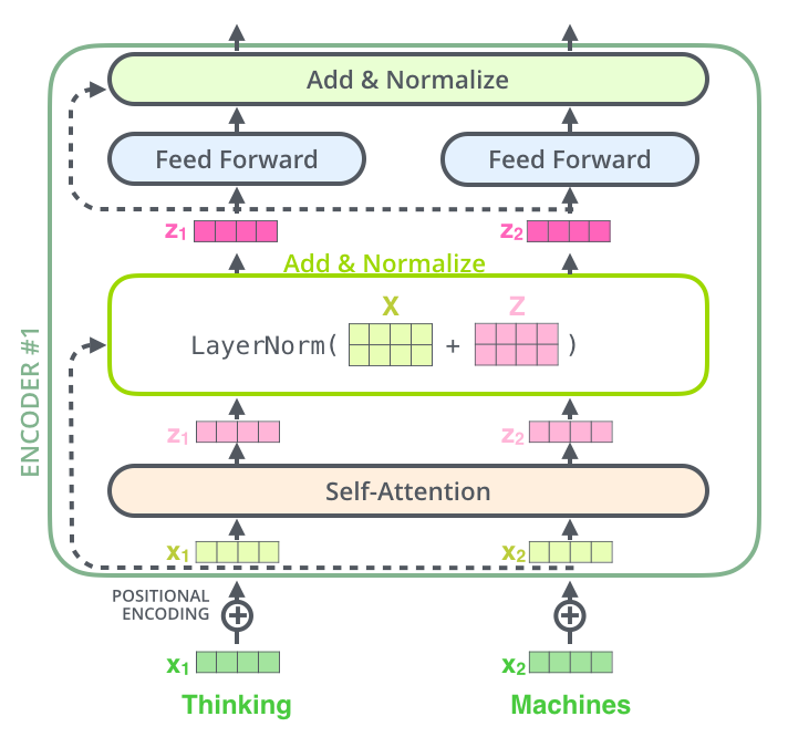
在Encoder之间会有残差连接,具体可以如下:
由上图可以看出残差连接会从下面的一个Self-Attention的输入连接到Self-Attention的输出进行 A d d 和 N o r m a l i z e Add和Normalize Add和Normalize操作,具体如下图所示:
同时解码器也有同样的结构,具体的可以用下图来表示:
2.8 解码器工作
编码器以处理输入序列作为开始,最顶端的编码器输出的 Q , K , V Q,K,V Q,K,V会送入解码器的每一个 E n c o d e r − D e c o d e r A t t e n t i o n Encoder-Decoder\,Attention Encoder−DecoderAttention层,从而能让解码器注意到适当的位置。

由上图可以看出,解码器的工作方式和编码器有些不同,解码器每一步输出一个元素,并重复这个过程直到输出一个特定的符号来表示一个翻译的结尾。,每一步的输出在下一次运算时被送入底部的解码器,并且项编码器一样被加入了位置信息。
Decoder中的Self-Attention层和Decoder中的有一些的区别,在Decoder中,self-attention layer 仅仅能访问之前输出的Output,这是通过在self-attenion 计算过程中Softmax步骤之前就把后面的位置填充为 − i n f -inf −inf符号来实现的。
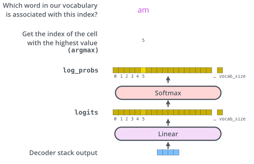
2.9 最后的Linear 和Softmax Layer
解码器把输出堆叠为浮点型向量,这个向量通过Linear层后跟Softmax layer 来实现的。通过Softmax layer算的对数概率,最后输出概率最大的那个单词。
3. 训练的一些细节
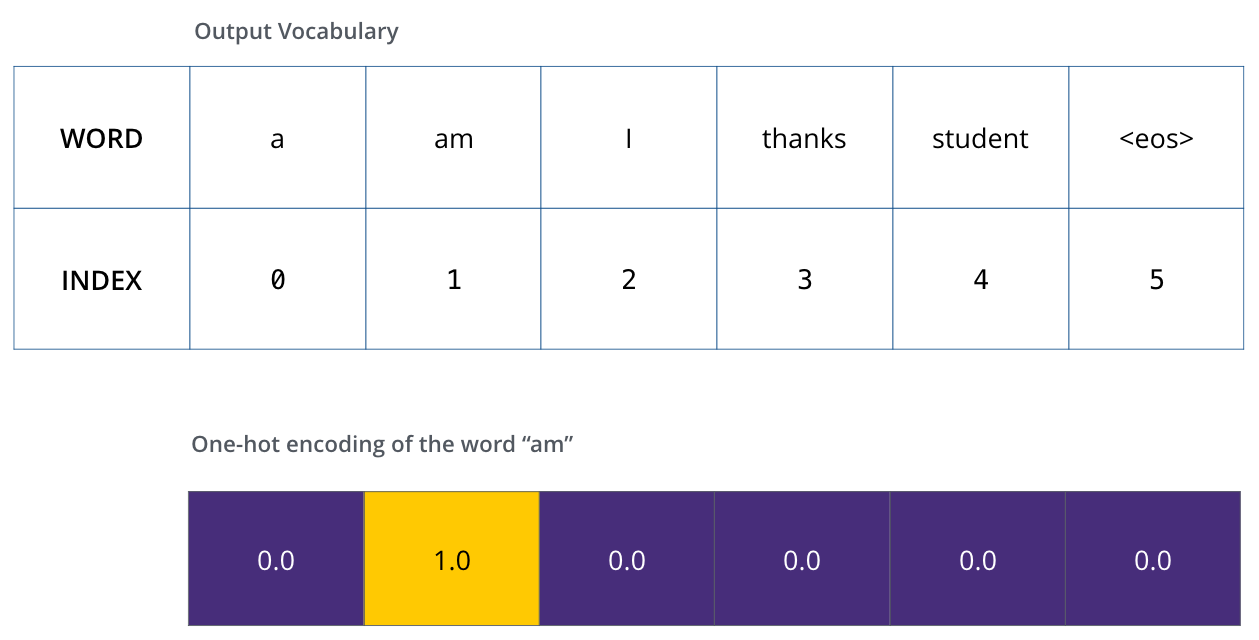
在训练过程中,可以把标注和输出进行监督学习.为了可视化这个过程,假设输出词汇仅包含六个单词(“a”, “am”, “i”, “thanks”, “student”, and “(eos是句子的结束符号)” ).
没有训练的输出可以比较杂乱无章, 他们之间的 l o s s loss loss就可以用一些交叉熵和KL散度等其他的方式来计算.
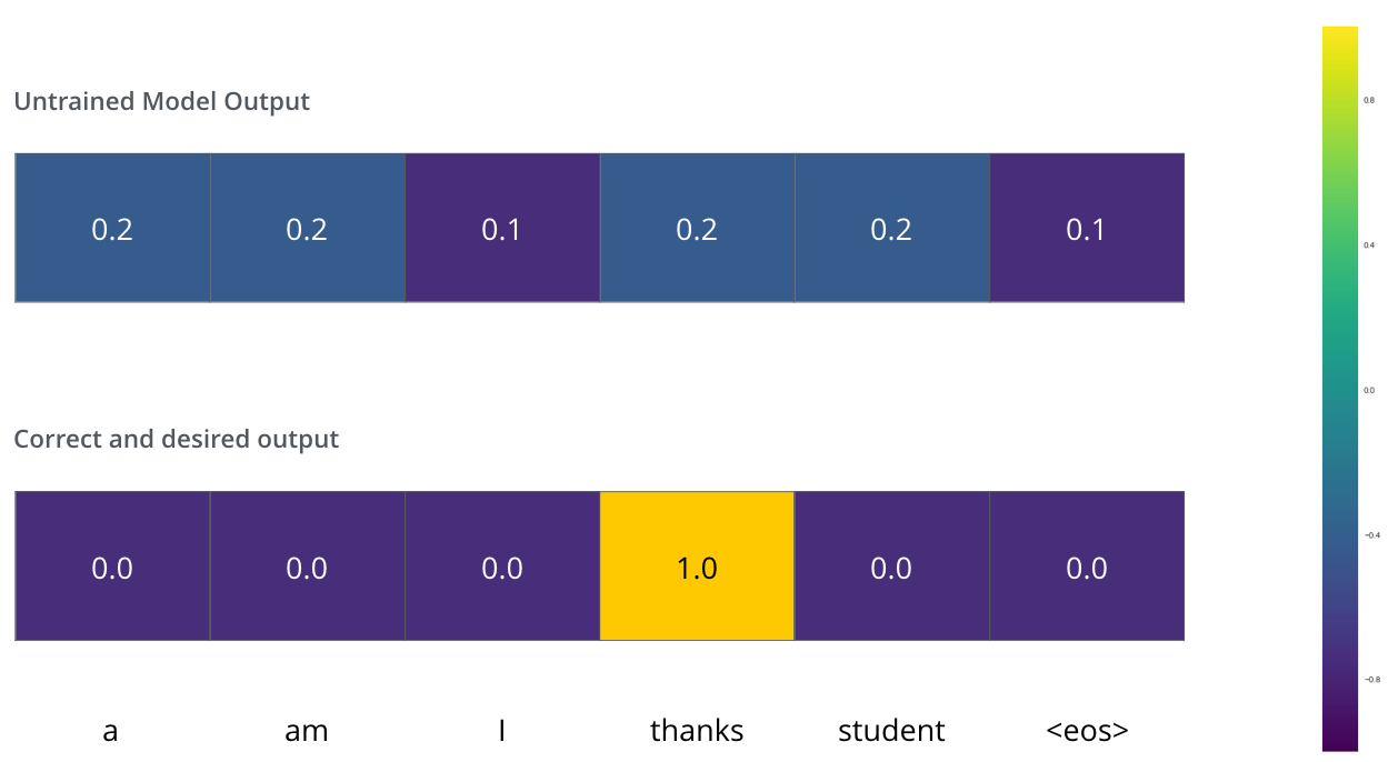
在经历过多次的迭代优化后,可以让其在对应的位置达到很高的概率.
4.参考资料
- 读 Attention Is All You Need 这一篇论文, the Transformer blog post (Transformer: A Novel Neural Network Architecture for Language Understanding), and the Tensor2Tensor announcement.
- 观看 Łukasz Kaiser’s talk 从而获得模型和细节
- 实战操作 Jupyter Notebook provided as part of the Tensor2Tensor repo
- 探索 Tensor2Tensor repo.
后续的一些工作:
- Depthwise Separable Convolutions for Neural Machine Translation
- One Model To Learn Them All
- Discrete Autoencoders for Sequence Models
- Generating Wikipedia by Summarizing Long Sequences
- Image Transformer
- Training Tips for the Transformer Model
- Self-Attention with Relative Position Representations
- Fast Decoding in Sequence Models using Discrete Latent Variables
- Adafactor: Adaptive Learning Rates with Sublinear Memory Cost


 3095
3095


 被折叠的 条评论
为什么被折叠?
被折叠的 条评论
为什么被折叠?
 到【灌水乐园】发言


