


文章目录
2.1 Harris角点监测器
Harris角点检测算法的主要思想:如果像素周围显示存在多于一个方向的边,则该点即为角点。
将图像域 中点 x上的对称半正定矩阵M1=M1(x)定义为:
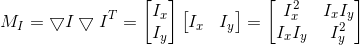
则M1的秩为1。对于图像的每一个像素,都可以计算得出该矩阵。
选择权重矩阵W(通常是高斯滤波器),可以得到卷积:
这个卷积的目的是得到M1在周围像素上的局部平均。计算得到的矩阵有称为Harris矩阵。W的宽度决定了在像素X周围的感兴趣区域。像这样在区域附近对Harris矩阵取平均的原因是,特征值会依赖于局部图像特性而变化。如果图像的梯度在该区域变化,那么harris矩阵的第二个特征值不再为0.如果图像的梯度没有变化,则特征值也不变。
取决于该区域梯度的值,Harris矩阵的特征值有三种情况:
1,如果两个特征值都是很大的正数,则该点为角点。
2,如果一个特征值很大,另一个约等于0,则该区域内存在一个边,区域内平均M1的特征值不会变化太大;
3,如果两个特征值都约等于0,该区域为空。
Harris角点检测程序:对于这个函数,使用高斯导数滤波器来计算导数,因为需要在角点检测过程中抑制噪声强度。
首先编辑自定义角点响应函数:
from scipy.ndimage import filters
from PIL import Image
from pylab import *
from numpy import *


def comput_harris_response(im, sigma=3):

    imx = zeros(im.shape)
    filters.gaussian_filter(im, (sigma, sigma), (0, 1), imx)
    imy = zeros(im.shape)
    filters.gaussian_filter(im, (sigma, sigma), (1, 0), imy)

    Wxx = filters.gaussian_filter(imx * imx, sigma)
    Wxy = filters.gaussian_filter(imx * imy, sigma)
    Wyy = filters.gaussian_filter(imy * imy, sigma)

    Wdet = Wxx*Wyy-Wxy**2
    Wtr = Wxx-Wyy

    return Wdet/Wtr
参数sigma定义了使用的高斯滤波器的尺度大小,可以修改sigma来尝试平均操作中的不同尺度,来计算harris矩阵
再从图像中挑选出需要的信息(选取像素值高于阈值的所有图像点,角点之间的间隔必须大于设定的最小距离。)
def get_harris_points(harrisim,min_dist=10,threshold=0.1):

  corner_threshold = harrisim.max() * threshold
  harrisim_t=(harrisim>corner_threshold)*1

  coords = array( harrisim_t.nonzero()).T

  candidate_values = [harrisim[c[0],c[1]] for c in coords]
  index = argsort(candidate_values)

  allowed_locations=zeros(harrisim.shape)
  allowed_locations[min_dist:-min_dist,min_dist:-min_dist]=1

  filtered_coords = []
    for i in index:
      if allowed_locations[coords[i, 0],coords[i,1]] ==1:
         filtered_coords.append(coords[i])
         allowed_locations[(coords[i, 0] - min_dist):(coords[i, 0] + min_dist),
         (coords[i, 1] - min_dist):(coords[i, 1] + min_dist)] = 0
  return filtered_coords
使用matplotlib模块绘制函数,
def plot_harris_points(image,filtered_coords):

    figure()
    gray()
    imshow(image)
    plot([p[1] for p in filtered_coords],[p[0] for p in filtered_coords],'*')
    axis('off')
    show()
自定义函数结束,调用函数,进行harris角点检测
im = array(Image.open('C:\\experiment\\test1.jpg').convert('L'))
harrisim = comput_harris_response(im)
filtered_coords = get_harris_points(harrisim,6)
plot_harris_points(im,filtered_coords)
设定阈值分别为0.1,0.01,0.001得到的结果分别为
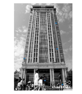
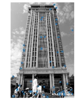
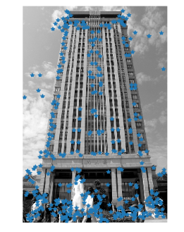
进行角点检测时,随着阈值的降低,能被检测到的角点相应大大增加。利用矩形窗在图像上移动,若窗内包含有角点,则窗口向各个方向移动时,窗内的灰度值都会发生变化。从而达到检测图像角点的目的。
在图像间寻找对应点
Harris角点检测仅仅能检测出图像中的兴趣点,但是没有给出通过比较图像间的兴趣点来寻找匹配角点的方法。需要在每个点上增加描绘子信息。
兴趣点描绘子是分配给兴趣点的一个向量,描绘该点附近的图像的表观信息。
Harris角点的描述子通常是由周围图像像素块的灰度值,以及用于比较的归一化互相关矩阵构成的。图像的像素块由以该像素点为中心的周围矩阵部分图像构成。
通常,两个(相同大小)像素块I1(x)和I2(x)的相关矩阵定义为:
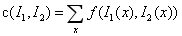
其中,函数f随着相关方法的变化而变化。上式取像素块中所有像素位置x的和。
def get_descriptors(image,filtered_coords,wid=5):

    desc=[]
    for coords in filtered_coords:
        patch = image[coords[0]-wid:coords[0]+wid+1,
                coords[1]-wid:coords[1]+wid+1].flatten()
        desc.append(patch)
        return desc
这个函数的参数是奇数大小长度的方形灰度图像块,该图像块的中心为处理的像素点。该函数将图像块像素值压平成一个向量,然后添加到描述子列表中。下面函数使用归一化的互相关矩阵,将每个描述子匹配道另一个图像的最优的候选点。
def match(desc1, desc2, threshold=0.5):
    n = len(desc1[0])
    d = -ones((len(desc1), len(desc2)))
    for i in range(len(desc2)):
        for j in range(len(desc2)):
            d1 = (desc1[i]-mean(desc1[i]))/std(desc1[i])
            d2 = (desc2[j]-mean(desc2[j]))/std(desc2[j])
            ncc_value = sum(d1*d2)/(n-1)
            if ncc_value > threshold:
                d[i, j] = ncc_value
    ndx = argsort(-d)
    matchscores = ndx[:, 0]

    return matchscores
为了获得稳定的匹配,两幅图像相互匹配,过滤不都是最好匹配的。(数值较高的距离代表两个点能更好地匹配。)代码如下:
def match_twosided(desc1,desc2,threshold=0.5):

    matches_12 = match(desc1, desc2, threshold)
    matches_21 = match(desc2, desc1, threshold)

    ndx_12 = where(matches_12 >= 0)[0]

    for n in ndx_12:
        if matches_21[matches_12[n]] != n:
            matches_12[n] = -1

    return matches_12
这些匹配可以通过在两边分别绘制图像,使用线段连接匹配的像素点来直观可视化。
def appendimages(im1,im2):

    rows1 = im1.shape[0]
    rows2 = im2.shape[0]

    if rows1 < rows2:
        im1 = concatenate((im1,zeros((rows2-rows1,im1.shape[1]))),axis=0)
    elif rows1 > rows2:
        im2 = concatenate((im2, zeros((rows1 - rows2, im2.shape[1]))), axis=0)

    return concatenate((im1, im2), axis=1)


def plot_matches(im1,im2,locs1,locs2,matchscores,show_below=True):

    im3 = appendimages(im1, im2)
    if show_below:
        im3 = vstack((im3, im3))

    imshow(im3)

    cols1 = im1.shape[1]
    for  i,m in enumerate(matchscores):
        if m>0:
            plot([locs1[i][1],locs2[m][1]+cols1],[locs1[i][0]],locs2[m][0],'c')
    axis('off')
运用自定义函数进行匹配
from PIL import Image
from numpy import *
from pylab import *
from PCV.localdescriptors import harris

imname='shangdalou.jpg'
im1=array(Image.open(imname).convert('L'))
im2=array(Image.open(imname).convert('L'))
wid=5
harrisim = harris.compute_harris_response(im1, 5)
filtered_coords1 = harris.get_harris_points(harrisim,wid+1)
d1 = harris.get_descriptors(im1,filtered_coords1,wid)

harrisim = harris.compute_harris_response(im2, 5)
filtered_coords2 = harris.get_harris_points(harrisim,wid+1)
d2 = harris.get_descriptors(im2,filtered_coords2,wid)

print 'starting matching'
matches=harris.match_twosided(d1,d2)

figure()
gray()
harris.plot_matches(im1,im2,filtered_coords1,filtered_coords2,matches)
show()

但是算法的结果存在一些不正确匹配,因为与现代的方法相比,像素块的互相关矩阵具有较弱的描述性。描述符不具有尺度不变性和旋转不变性,而算法中像素块的大小也会影响对应匹配的结果。尺度不变特征变换(SIFT)算法能够提高特征点检测和描述性能。
2.2 SIFT(尺度不变特征变换)
SIFT特征包括兴趣点检测器和描述子。SIFT描述子具有非常强的稳健性,对于尺度,旋转和亮度都具有不变性。
SIFT算法的特点有:
-
SIFT特征是图像的局部特征,其对旋转、尺度缩放、亮度变化保持不变性,对视角变化、仿射变换、噪声也保持一定程度的稳定性;
-
独特性(Distinctiveness)好,信息量丰富,适用于在海量特征数据库中进行快速、准确的匹配;
-
多量性,即使少数的几个物体也可以产生大量的SIFT特征向量;
-
高速性,经优化的SIFT匹配算法甚至可以达到实时的要求;
-
可扩展性,可以很方便的与其他形式的特征向量进行联合。
SIFT算法可以解决的问题:
目标的自身状态、场景所处的环境和成像器材的成像特性等因素影响图像配准/目标识别跟踪的性能。而SIFT算法在一定程度上可解决:
-
目标的旋转、缩放、平移(RST)
-
图像仿射/投影变换(视点viewpoint)
-
光照影响(illumination)
-
目标遮挡(occlusion)
-
杂物场景(clutter)
-
噪声
SIFT算法的实质是在不同的尺度空间上查找关键点(特征点),并计算出关键点的方向。SIFT所查找到的关键点是一些十分突出,不会因光照,仿射变换和噪音等因素而变化的点,如角点、边缘点、暗区的亮点及亮区的暗点等。
Lowe将SIFT算法分解为如下四步:
-
尺度空间极值检测:搜索所有尺度上的图像位置。通过高斯微分函数来识别潜在的对于尺度和旋转不变的兴趣点。
-
关键点定位:在每个候选的位置上,通过一个拟合精细的模型来确定位置和尺度。关键点的选择依据于它们的稳定程度。
-
方向确定:基于图像局部的梯度方向,分配给每个关键点位置一个或多个方向。所有后面的对图像数据的操作都相对于关键点的方向、尺度和位置进行变换,从而提供对于这些变换的不变性。
-
关键点描述:在每个关键点周围的邻域内,在选定的尺度上测量图像局部的梯度。这些梯度被变换成一种表示,这种表示允许比较大的局部形状的变形和光照变化。(摘录自http://blog.csdn.net/zddblog/article/details/7521424)详情见http://blog.csdn.net/zddblog/article/details/7521424
2.2.1 兴趣点
SIFT特征使用高斯差分函数来定位兴趣点:

兴趣点是在图像位置和尺度变化下计算结果的最大值和最小值点。这些候选点通过滤波去除不稳定点。基于一些准则,比如认为低对比度和位于边上的点不是兴趣点,可以再去除一些候选的兴趣点。
2.2.2 描述子
上面讨论的兴趣点位置描述子给出了兴趣点的位置和尺度信息。为了实现旋转不变性,基于每个点周围图像梯度的方向和大小,sift描述子又引入了参考方向。SIFT描述子使用主方向描述参考方向。主方向使用方向直方图(以大小为权重)来度量。
为了对图像具有稳健性,SIFT描述子使用图像梯度,SIFT描述子在每个像素点附近选取子区域网格,在每个子区域内计算图像梯度方向直方图。每个子区域的直方图拼接起来组成描述子向量。SIFT描述子的标准设置使用4*4的子区域,每个子区域使用8个小区间的方向直方图,会产生128个小区间的直方图。
2.2.3 检测兴趣点
使用开源工具包VLFEAT提供的二进制文件来计算图像的SIFT特征。(具体操作:下载vlfeat-0.9.20-bin版本,将bin 目录下的sift.exe,以及vl.dll拷贝到py文件的平行目录中)。
调用PCV包里面的sift.py文件,完成兴趣点的检测
from PIL import Image
from numpy import *
from pylab import *
from PCV.localdescriptors import sift

imname = 'shangdalou.jpg'
im1=array(Image.open(imname).convert('L'))
sift.process_image(imname,'shangdalou.sift')
l1,d1=sift.read_features_from_file('shangdalou.sift')

figure()
gray()
sift.plot_features(im1,l1,circle=True)
show()

将sift特征图片与harris角点进行比较,可以看到两个算法所选的特征点是不同的。IFT选取的对象会使用DoG检测关键点,并且对每个关键点周围的区域计算特征向量,它主要包括两个操作:检测和计算,操作的返回值是关键点信息和描述符,最后在图像上绘制关键点,并用imshow函数显示这幅图像。
2.2.4 匹配描述子
对于将一幅图像中的特征匹配到另外一幅图像的特征,一种稳定的准则是使用这两个特征距离和两个最匹配的特征距离的比率。相比于图像中的其他特征,该准则保证能够找到足够相似的唯一特征。
与harris方法相同处在于,匹配描述子也是进行两次,分别从第一幅匹配第二幅,第二幅匹配第一幅,去掉不都是最佳匹配的点。
2.3 匹配地理标记图像
2.3.2 使用局部描述子匹配
首先对下载的图像提取局部描述子。用sift特征提取代码对图像进行处理,并将特征保存在和图像同名(.sift)的文件中。对所有组合图像进行逐个匹配。
import sift
nbr_images = len(imlist)
matchscores = zeros((nbr_images,nbr_images))
for i in range(nbr_images):
 for j in range(i,nbr_images): # 仅仅计算上三角
 print 'comparing ', imlist[i], imlist[j]
 l1,d1 = sift.read_features_from_file(featlist[i])
 l2,d2 = sift.read_features_from_file(featlist[j])
 matches = sift.match_twosided(d1,d2)
 nbr_matches = sum(matches > 0)
 print 'number of matches = ', nbr_matches
 matchscores[i,j] = nbr_matches
 # 复制值
 for i in range(nbr_images):
 for j in range(i+1,nbr_images): # 不需要复制对角线
 matchscores[j,i] = matchscores[i,j]
将每对图像间的匹配特征数保存在matchscores数组。
662 0 0 2 0 0 0 0 1 0 0 1 2 0 3 0 19 1 0 2
0 901 0 1 0 0 0 1 1 0 0 1 0 0 0 0 0 0 1 2
0 0 266 0 0 0 0 0 0 0 0 0 0 1 0 0 0 0 0 0
2 1 0 1481 0 0 2 2 0 0 0 2 2 0 0 0 2 3 2 0
0 0 0 0 1748 0 0 1 0 0 0 0 0 2 0 0 0 0 0 1
0 0 0 0 0 1747 0 0 1 0 0 0 0 0 0 0 0 1 1 0
0 0 0 2 0 0 555 0 0 0 1 4 4 0 2 0 0 5 1 0
0 1 0 2 1 0 0 2206 0 0 0 1 0 0 1 0 2 0 1 1
1 1 0 0 0 1 0 0 629 0 0 0 0 0 0 0 1 0 0 20
0 0 0 0 0 0 0 0 0 829 0 0 1 0 0 0 0 0 0 2
0 0 0 0 0 0 1 0 0 0 1025 0 0 0 0 0 1 1 1 0
1 1 0 2 0 0 4 1 0 0 0 528 5 2 15 0 3 6 0 0
2 0 0 2 0 0 4 0 0 1 0 5 736 1 4 0 3 37 1 0
0 0 1 0 2 0 0 0 0 0 0 2 1 620 1 0 0 1 0 0
3 0 0 0 0 0 2 1 0 0 0 15 4 1 553 0 6 9 1 0
0 0 0 0 0 0 0 0 0 0 0 0 0 0 0 2273 0 1 0 0
19 0 0 2 0 0 0 2 1 0 1 3 3 0 6 0 542 0 0 0
1 0 0 3 0 1 5 0 0 0 1 6 37 1 9 1 0 527 3 0
0 1 0 2 0 1 1 1 0 0 1 0 1 0 1 0 0 3 1139 0
2 2 0 0 1 0 0 1 20 2 0 0 0 0 0 0 0 0 0 499
使用该 matchscores 矩阵作为图像间简单的距离度量方式(具有相似内容的图像
间拥有更多的匹配特征数),下面我们可以使用相似的视觉内容来将这些图像连接
起来。
2.3.3 可视化连接的图像
使用pydot工具包,创建一个可视化的连接图。代码如下:
import pydot

g = pydot.Dot(graph_type='graph')
g.add_node(pydot.Node(str(0),fontcolor='transparent'))

for i in range(5):
  g.add_node(pydot.Node(str(i+1)))
  g.add_edge(pydot.Edge(str(0),str(i+1)))
  for j in range(5):
   g.add_node(pydot.Node(str(j+1)+'-'+str(i+1)))
   g.add_edge(pydot.Edge(str(j+1)+'-'+str(i+1),str(j+1)))
g.write_png('graph.jpg',prog='neato')
得到的结果:

为了创建显示可能图像组的图,如
果匹配的数目高于一个阈值,我们使用边来连接相应的图像节点。为了得到图中的
图像,需要使用图像的全路径(在下面例子中,使用 path 变量表示)。为了使图像
看起来漂亮,我们需要将每幅图像尺度化为缩略图形式,缩略图的最大边为 100 像
素。下面是具体实现代码:
# -*- coding: utf-8 -*-
import json
import os
import urllib
import urlparse
from pylab import *
from PIL import Image
from PCV.localdescriptors import sift
from PCV.tools import imtools
import pydot

download_path = "C:\\Users\\xqm\\PycharmProjects\\sucai"
path = "C:\\Users\\xqm\\PycharmProjects\\sucai\\"

imlist = imtools.get_imlist(download_path)
nbr_images = len(imlist)

featlist = [imname[:-3] + 'sift' for imname in imlist]
for i, imname in enumerate(imlist):
    sift.process_image(imname, featlist[i])

matchscores = zeros((nbr_images, nbr_images))

for i in range(nbr_images):
    for j in range(i, nbr_images):  # only compute upper triangle
        print('comparing ', imlist[i], imlist[j])
        l1, d1 = sift.read_features_from_file(featlist[i])
        l2, d2 = sift.read_features_from_file(featlist[j])
        matches = sift.match_twosided(d1, d2)
        nbr_matches = sum(matches > 0)
        print('number of matches = ', nbr_matches)
        matchscores[i, j] = nbr_matches

# copy values
for i in range(nbr_images):
    for j in range(i + 1, nbr_images):  # no need to copy diagonal
        matchscores[j, i] = matchscores[i, j]

# 可视化

threshold = 2  # min number of matches needed to create link

g = pydot.Dot(graph_type='graph')  # don't want the default directed graph

for i in range(nbr_images):
    for j in range(i + 1, nbr_images):
        if matchscores[i, j] > threshold:
            # first image in pair
            im = Image.open(imlist[i])
            im.thumbnail((100, 100))
            filename = path + str(i) + '.jpg'
            im.save(filename)  # need temporary files of the right size
            g.add_node(pydot.Node(str(i), fontcolor='transparent', shape='rectangle', image=filename))

            # second image in pair
            im = Image.open(imlist[j])
            im.thumbnail((100, 100))
            filename = path + str(j) + '.jpg'
            im.save(filename)  # need temporary files of the right size
            g.add_node(pydot.Node(str(j), fontcolor='transparent', shape='rectangle', image=filename))

            g.add_edge(pydot.Edge(str(i), str(j)))
g.write_jpg('jimei.jpg')
代码运行的结果:
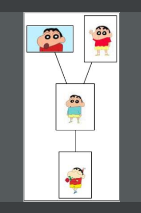
在文件夹中存放了五张图像,其中四幅匹配成功显示,并实现了可视性连接,余下一幅差异太大。


 324
324


 被折叠的 条评论
为什么被折叠?
被折叠的 条评论
为什么被折叠?
 到【灌水乐园】发言


