


文章目录
YoloV3相比V2的改进点
1、New structure
作用:为了速度更快
2、Multiscale Structure
3 scales; 3 anchors per scale per grid
/32,small scale (13 x 13) —> large anchor
/16,mid scale (26 x 26) —> medium anchor
/8,large scale (52 x 52) —> small anchor
3、Change Classification
80 classes, from softmax —> logistic
----------------------------------------------------------------------------------------
YoloV3代码解析
一、网络结构
1、主干网络(backbone)
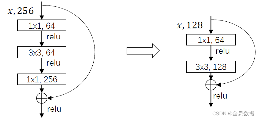
YoloV3的主干网络是darknet53网络,用于特征提取和特征融合,主要用到了 1×1 和 3×3 的卷积,
以及改进的resnet,如图:
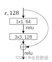
下面的结构图把darknet53网络完整地表现了出来,参考链接
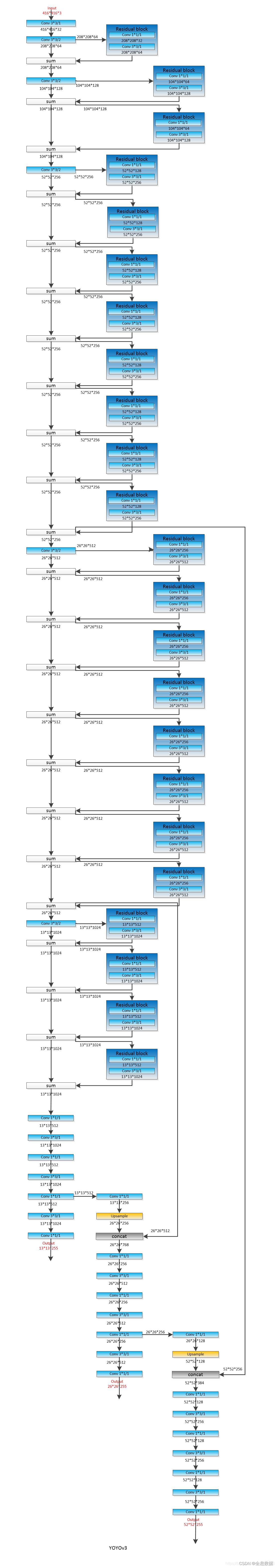
主干网络的参数:
# [] 往往是layer name
[net]
# Testing
#batch=1
#subdivisions=1
# Training
# batch & subdivision: real training size each time: batch/subdivisions
# yolov4 creates a newer CmBN method based on this)
batch = 16  # 和其他项目中的batch_size是一个意思
# 历史遗留问题,当时硬件不行,所以有时候用batch/subdivisions分批处理,然后再把这些部分拼接起来
subdivisions = 1
width = 416
height = 416
channels = 3

# 优化器相关的参数
momentum = 0.9
decay = 0.0005
# Optimizer:
# *** 面试前必须要会的 *** ,’||‘前后的优化机理不一致
# please remember SGD(+ Momentum), Nesterov, RMSProp || Adagrad, Adam & then:
#
# Better to know AdamW. 至少会一个
# AdamW: paper:  https://arxiv.org/pdf/1711.05101.pdf (decoupled weight decay regularization) +
#        github: https://github.com/ShikamaruZhang/AdamW
# Nadam: http://cs229.stanford.edu/proj2015/054_report.pdf [not a paper, a course report]
# RAdam: https://arxiv.org/pdf/1908.03265.pdf
# LookAhead: https://arxiv.org/abs/1907.08610
# Ranger: (RAdam + LookAhead + GC [Gradient Centralization]) https://github.com/lessw2020/Ranger-Deep-Learning-Optimizer
#         work with Mish (activation function) perfectly
# LAMB (BERT, Both large(>1k) & regular batch size): https://arxiv.org/pdf/1904.00962.pdf

# for data augmentation (angle is not used in program): color shifting
# jitter=.3 (in [yolo] section) is also used for data augmentation: size of original image
# 数据增广相关的参数
angle = 0
saturation = 1.5
exposure = 1.5
hue = .1

learning_rate = 0.001
# BURN_IN:
# Worked in original Darknet. We may have training policy to change the lr.
# We start this procedure after burn_in. So, before burn_in: policy0, after burn_in: policy we set (like multi-step)
# Usually, we set lr from 0 to initial lr during burn-in
#
# If we use SGD, a good implementation:
# https://github.com/ultralytics/yolov3/commit/a722601ef61149cc9e5135f58c762310627c970a [line 115-124]
#
# Another good example to burn-in (here we use: warmup, same thing):
# Faceboxes: https://github.com/zisianw/FaceBoxes.PyTorch/blob/master/train.py (from line 137)
#
# So, initial LR you set should not be too far away from the last value after burn-in
#
# Why burn-in:
# RAdam's explanation: The core issue is that adaptive learning rate optimizers have too large of a variance,
# especially in the early stages of training, and make excessive jumps based on limited training data. Therefore,
# warmup serves as a variance reduce
# [Cannot explain why SGD+warmup can also present better effect]
# [Just like you enter in a new environment, you also need time to warmup]
# [The use of burn-in/warmup can be dated back to ResNet)]
# 效果并不是很明显,没有理论依据,意思是从0到0.001线性迭代1000次
burn_in = 1000
# warm up 更新策略
max_batches = 500200
policy = steps
steps = 400000,450000
scales = .1,.1

# A very good figural explanation:
# https://blog.csdn.net/dz4543/article/details/90049377

# *** backbone ***
# layer 0
[convolutional]
batch_normalize = 1
# 输出channel个数
filters = 32
size = 3
stride = 1
pad = 1
# leaky=leaky relu
activation = leaky

# Downsample
# layer 1
[convolutional]
batch_normalize = 1
filters = 64
size = 3
stride = 2
pad = 1
activation = leaky
# layer 2
[convolutional]
batch_normalize = 1
filters = 32
size = 1
stride = 1
pad = 1
activation = leaky
# layer 3
[convolutional]
batch_normalize = 1
filters = 64
size = 3
stride = 1
pad = 1
activation = leaky
# 4 = 1(4-3) + 3(上一层)
[shortcut]
# output = network[-3] + network[shortcut/current]
# linear: do nothing. 占位用
from = -3
activation = linear

# Downsample
# 5
[convolutional]
batch_normalize = 1
filters = 128
size = 3
stride = 2
pad = 1
activation = leaky
# 6
[convolutional]
batch_normalize = 1
filters = 64
size = 1
stride = 1
pad = 1
activation = leaky
# 7
[convolutional]
batch_normalize = 1
filters = 128
size = 3
stride = 1
pad = 1
activation = leaky
# 8 = 5 + 7
[shortcut]
from = -3
activation = linear
# 9
[convolutional]
batch_normalize = 1
filters = 64
size = 1
stride = 1
pad = 1
activation = leaky
# 10
[convolutional]
batch_normalize = 1
filters = 128
size = 3
stride = 1
pad = 1
activation = leaky
# 11 = 8 + 10
[shortcut]
from = -3
activation = linear

# Downsample
# 12
[convolutional]
batch_normalize = 1
filters = 256
size = 3
stride = 2
pad = 1
activation = leaky
# 13
[convolutional]
batch_normalize = 1
filters = 128
size = 1
stride = 1
pad = 1
activation = leaky
# 14
[convolutional]
batch_normalize = 1
filters = 256
size = 3
stride = 1
pad = 1
activation = leaky
# 15 = 12 + 14
[shortcut]
from = -3
activation = linear
# 16
[convolutional]
batch_normalize = 1
filters = 128
size = 1
stride = 1
pad = 1
activation = leaky
# 17
[convolutional]
batch_normalize = 1
filters = 256
size = 3
stride = 1
pad = 1
activation = leaky
# 18 = 15 + 17
[shortcut]
from = -3
activation = linear
# 19
[convolutional]
batch_normalize = 1
filters = 128
size = 1
stride = 1
pad = 1
activation = leaky
# 20
[convolutional]
batch_normalize = 1
filters = 256
size = 3
stride = 1
pad = 1
activation = leaky
# 21 = 18 + 20
[shortcut]
from = -3
activation = linear
# 22
[convolutional]
batch_normalize = 1
filters = 128
size = 1
stride = 1
pad = 1
activation = leaky
# 23
[convolutional]
batch_normalize = 1
filters = 256
size = 3
stride = 1
pad = 1
activation = leaky
# 24 = 21 + 23
[shortcut]
from = -3
activation = linear
# 25
[convolutional]
batch_normalize = 1
filters = 128
size = 1
stride = 1
pad = 1
activation = leaky
# 26
[convolutional]
batch_normalize = 1
filters = 256
size = 3
stride = 1
pad = 1
activation = leaky
# 27 = 24 + 26
[shortcut]
from = -3
activation = linear
# 28
[convolutional]
batch_normalize = 1
filters = 128
size = 1
stride = 1
pad = 1
activation = leaky
# 29
[convolutional]
batch_normalize = 1
filters = 256
size = 3
stride = 1
pad = 1
activation = leaky
# 30 = 27 + 29
[shortcut]
from = -3
activation = linear
# 31
[convolutional]
batch_normalize = 1
filters = 128
size = 1
stride = 1
pad = 1
activation = leaky
# 32
[convolutional]
batch_normalize = 1
filters = 256
size = 3
stride = 1
pad = 1
activation = leaky
# 33 = 30 + 32
[shortcut]
from = -3
activation = linear
# 34
[convolutional]
batch_normalize = 1
filters = 128
size = 1
stride = 1
pad = 1
activation = leaky
# 35
[convolutional]
batch_normalize = 1
filters = 256
size = 3
stride = 1
pad = 1
activation = leaky
# 36 = 33 + 35
[shortcut]
from = -3
activation = linear

# Downsample
# 37
[convolutional]
batch_normalize = 1
filters = 512
size = 3
stride = 2
pad = 1
activation = leaky
# 38
[convolutional]
batch_normalize = 1
filters = 256
size = 1
stride = 1
pad = 1
activation = leaky
# 39
[convolutional]
batch_normalize = 1
filters = 512
size = 3
stride = 1
pad = 1
activation = leaky
# 40 = 37 + 39
[shortcut]
from = -3
activation = linear

# 41
[convolutional]
batch_normalize = 1
filters = 256
size = 1
stride = 1
pad = 1
activation = leaky
# 42
[convolutional]
batch_normalize = 1
filters = 512
size = 3
stride = 1
pad = 1
activation = leaky
# 43 = 40 + 42
[shortcut]
from = -3
activation = linear

# 44
[convolutional]
batch_normalize = 1
filters = 256
size = 1
stride = 1
pad = 1
activation = leaky
# 45
[convolutional]
batch_normalize = 1
filters = 512
size = 3
stride = 1
pad = 1
activation = leaky
# 46 = 43 + 45
[shortcut]
from = -3
activation = linear

# 47
[convolutional]
batch_normalize = 1
filters = 256
size = 1
stride = 1
pad = 1
activation = leaky
# 48
[convolutional]
batch_normalize = 1
filters = 512
size = 3
stride = 1
pad = 1
activation = leaky
# 49 = 46 + 48
[shortcut]
from = -3
activation = linear
# 50
[convolutional]
batch_normalize = 1
filters = 256
size = 1
stride = 1
pad = 1
activation = leaky
# 51
[convolutional]
batch_normalize = 1
filters = 512
size = 3
stride = 1
pad = 1
activation = leaky
# 52 = 49 + 51
[shortcut]
from = -3
activation = linear

# 53
[convolutional]
batch_normalize = 1
filters = 256
size = 1
stride = 1
pad = 1
activation = leaky
# 54
[convolutional]
batch_normalize = 1
filters = 512
size = 3
stride = 1
pad = 1
activation = leaky
# 55 = 52 + 54
[shortcut]
from = -3
activation = linear

# 56
[convolutional]
batch_normalize = 1
filters = 256
size = 1
stride = 1
pad = 1
activation = leaky
# 57
[convolutional]
batch_normalize = 1
filters = 512
size = 3
stride = 1
pad = 1
activation = leaky
# 58 = 55 + 57
[shortcut]
from = -3
activation = linear
# 59
[convolutional]
batch_normalize = 1
filters = 256
size = 1
stride = 1
pad = 1
activation = leaky
# 60
[convolutional]
batch_normalize = 1
filters = 512
size = 3
stride = 1
pad = 1
activation = leaky
# 61 = 58 + 60
[shortcut]
from = -3
activation = linear

# Downsample
# 62
[convolutional]
batch_normalize = 1
filters = 1024
size = 3
stride = 2
pad = 1
activation = leaky
# 63
[convolutional]
batch_normalize = 1
filters = 512
size = 1
stride = 1
pad = 1
activation = leaky
# 64
[convolutional]
batch_normalize = 1
filters = 1024
size = 3
stride = 1
pad = 1
activation = leaky
# 65 = 62 + 64
[shortcut]
from = -3
activation = linear
# 66
[convolutional]
batch_normalize = 1
filters = 512
size = 1
stride = 1
pad = 1
activation = leaky
# 67
[convolutional]
batch_normalize = 1
filters = 1024
size = 3
stride = 1
pad = 1
activation = leaky
# 68 = 65 + 67
[shortcut]
from = -3
activation = linear
# 69
[convolutional]
batch_normalize = 1
filters = 512
size = 1
stride = 1
pad = 1
activation = leaky
# 70
[convolutional]
batch_normalize = 1
filters = 1024
size = 3
stride = 1
pad = 1
activation = leaky
# 71 = 68 + 70
[shortcut]
from = -3
activation = linear
# 72
[convolutional]
batch_normalize = 1
filters = 512
size = 1
stride = 1
pad = 1
activation = leaky
# 73
[convolutional]
batch_normalize = 1
filters = 1024
size = 3
stride = 1
pad = 1
activation = leaky
# 74 = 71  + 73
[shortcut]
from = -3
activation = linear

######################
# 75

# *** 第1个neck ***

[convolutional]
batch_normalize = 1
filters = 512
size = 1
stride = 1
pad = 1
activation = leaky
# 76
[convolutional]
batch_normalize = 1
size = 3
stride = 1
pad = 1
filters = 1024
activation = leaky
# 77
[convolutional]
batch_normalize = 1
filters = 512
size = 1
stride = 1
pad = 1
activation = leaky
# 78
[convolutional]
batch_normalize = 1
size = 3
stride = 1
pad = 1
filters = 1024
activation = leaky
# 79
[convolutional]
batch_normalize = 1
filters = 512
size = 1
stride = 1
pad = 1
activation = leaky
# 80
[convolutional]
batch_normalize = 1
size = 3
stride = 1
pad = 1
filters = 1024
activation = leaky
# 81
[convolutional]
size = 1
stride = 1
pad = 1
# (classes + 1+ coords) * anchors_num = 85 * 3 = 255
filters = 255
activation = linear

# *** head ***

# 82
[yolo]
# 13x13 feature map,
# corresponding bigger object.
# Corresponding last 3 anchors
mask = 6,7,8
anchors = 10,13,  16,30,  33,23,  30,61,  62,45,  59,119,  116,90,  156,198,  373,326
classes = 80
# 一共有9个anchor
num = 9
# 没啥用
jitter = .3
# will be reset to 0.5 in models.py/YOLOLayer.init [will revisit later]
ignore_thresh = .7
truth_thresh = 1
# size changed from 320-608 randomly
random = 1

# 83 = 79
[route]
# go back to layer[-4]
# output(layer[-4])
layers = -4
# 84 (接从83,实际就是从79接)
[convolutional]
batch_normalize = 1
filters = 256
size = 1
stride = 1
pad = 1
activation = leaky
# 85
[upsample]
stride = 2
# 86 = concat(85, 61)
[route]
# output = concat(output(layers[-1]), output(layers[61]))
layers = -1, 61

# 第2个neck
# 87
[convolutional]
batch_normalize = 1
filters = 256
size = 1
stride = 1
pad = 1
activation = leaky
# 88
[convolutional]
batch_normalize = 1
size = 3
stride = 1
pad = 1
filters = 512
activation = leaky
# 89
[convolutional]
batch_normalize = 1
filters = 256
size = 1
stride = 1
pad = 1
activation = leaky
# 90
[convolutional]
batch_normalize = 1
size = 3
stride = 1
pad = 1
filters = 512
activation = leaky
# 91
[convolutional]
batch_normalize = 1
filters = 256
size = 1
stride = 1
pad = 1
activation = leaky
# 92
[convolutional]
batch_normalize = 1
size = 3
stride = 1
pad = 1
filters = 512
activation = leaky
# 93
[convolutional]
size = 1
stride = 1
pad = 1
filters = 255
activation = linear

# 94: 26 x 26 x 255, corresponding to the mid 3 anchors
[yolo]
mask = 3,4,5
anchors = 10,13,  16,30,  33,23,  30,61,  62,45,  59,119,  116,90,  156,198,  373,326
classes = 80
num = 9
jitter = .3
ignore_thresh = .7
truth_thresh = 1
random = 1


# 95 = 90
[route]
layers = -4
# 96 (从95,也就是90开始接)
[convolutional]
batch_normalize = 1
filters = 128
size = 1
stride = 1
pad = 1
activation = leaky
# 97
[upsample]
stride = 2
# 98 = concat(97, 36)
[route]
layers = -1, 36

# 第3个neck
# 99
[convolutional]
batch_normalize = 1
filters = 128
size = 1
stride = 1
pad = 1
activation = leaky
# 100
[convolutional]
batch_normalize = 1
size = 3
stride = 1
pad = 1
filters = 256
activation = leaky
# 101
[convolutional]
batch_normalize = 1
filters = 128
size = 1
stride = 1
pad = 1
activation = leaky
# 102
[convolutional]
batch_normalize = 1
size = 3
stride = 1
pad = 1
filters = 256
activation = leaky
# 103
[convolutional]
batch_normalize = 1
filters = 128
size = 1
stride = 1
pad = 1
activation = leaky
# 104
[convolutional]
batch_normalize = 1
size = 3
stride = 1
pad = 1
filters = 256
activation = leaky
# 105
[convolutional]
size = 1
stride = 1
pad = 1
filters = 255
activation = linear

# 106: 52 x 52 x 255, corresponding to first 3 anchors
[yolo]
mask = 0,1,2
anchors = 10,13,  16,30,  33,23,  30,61,  62,45,  59,119,  116,90,  156,198,  373,326
classes = 80
num = 9
jitter = .3
ignore_thresh = .7
truth_thresh = 1
random = 1
2、解析主干网络的参数
把上面主干网络的参数进行解析,输出格式为:[{“type”:xxx, “batch_normalize”:0, …}, …]
def parse_model_config(path):
    """返回每一个layer,并用一个字典来表示,即返回 [{net},{layer},{layer},..] """
    """Parses the yolo-v3 layer configuration file and returns module definitions"""
    file = open(path, 'r')  # 以读的方式打开文件
    # lines的输出格式为:['# 浼樺寲鍣ㄧ浉鍏崇殑鍙傛暟', 'momentum = 0.9', 'decay = 0.0005', ....]
    lines = file.read().split('\n')  # 直接读取文件中的字符
    # startswith:判断字符串是否以指定字符或子字符串开头
    lines = [x for x in lines if x and not x.startswith('#')]  # 去除掉所有空白行 与 #开头的行
    # 如果strip()的参数为空,那么会默认删除字符串头和尾的空白字符(包括\n,\r,\t这些)
    # rstrip().lstrip()的效果和strip()是一样的
    lines = [x.rstrip().lstrip() for x in lines]  # get rid of fringe whitespaces
    module_defs = []
    for line in lines:
        # 读入当前module的名字
        if line.startswith('['):  # This marks the start of a new block
            module_defs.append({})
            module_defs[-1]['type'] = line[1:-1].rstrip()  # 取出layer的类型,如:是convolutional还是yolo
            if module_defs[-1]['type'] == 'convolutional':
                module_defs[-1]['batch_normalize'] = 0  # 预存,防止某些层没有此参数 (只在3个yolo层前没有)
        # 读入当前module的参数
        else:
            key, value = line.split("=")
            value = value.strip()
            module_defs[-1][key.rstrip()] = value.strip()  # 去除掉"="左右两边的“ ”

    return module_defs
3、执行主干网络
执行解析后网络,代码较长,但一行一行的看是能看懂的,主要是执行convolutional、upsample、route、shortcut、以及yolo层,
def create_modules(module_defs):
    """我的理解:使用module_list存储每一个layer执行"""

    """
    Constructs module list of layer blocks from module configuration in module_defs
    """
    # module_defs = [{"type":"net", "channels":3, ...},                     # each element is a layer block (dtype=dict)
    #                {"type":"convolutional", "batch_normalize":1, ...},
    #                ...]

    hyperparams = module_defs.pop(0)  # 取出[net]的整体参数
    output_filters = [int(hyperparams["channels"])]  # 3: 最初。因为是rgb 3通道
    module_list = nn.ModuleList()  # 存储每一大层,如conv层: 包括conv-bn-leaky relu等
    # nn.ModuleList() & nn.Sequential()
    # nn.ModuleList(): 就是Module的list,并没有实现forward函数(并没有实际执行的函数),所以只是module的list,并不需要module之间的顺序
    #                  关系
    # nn.Sequential(): module的顺序执行。是实现了forward函数的,即会顺序执行其中的module,所以每个module的size必须匹配
    # 说的不错的链接:https://blog.csdn.net/watermelon1123/article/details/89954224
    #              https://zhuanlan.zhihu.com/p/64990232
    for module_i, module_def in enumerate(module_defs):
        modules = nn.Sequential()  # 存下每一大层的执行,如conv层: 包括conv-bn-leaky relu等
        if module_def["type"] == "convolutional":
            bn = int(module_def["batch_normalize"])
            filters = int(module_def["filters"])  # 输出channel个数
            kernel_size = int(module_def["size"])
            pad = (kernel_size - 1) // 2
            modules.add_module(
                f"conv_{module_i}",  # a newer formatting method for python3.x, called f-string. Better than %s..
                nn.Conv2d(
                    in_channels=output_filters[-1],
                    out_channels=filters,
                    kernel_size=kernel_size,
                    stride=int(module_def["stride"]),
                    padding=pad,
                    bias=not bn,  # not 1:False
                ),
            )
            if bn:
                # momentum:一个用于运行过程中均值和方差的一个估计参数,默认值为0.1
                # momentum:一个稳定系数, eps:分母中添加的一个值,目的是为了计算的稳定性,默认为:1e-5
                # https://blog.csdn.net/weixin_40522801/article/details/106185263?ops_request_misc=&request_id=&biz_id=102&utm_term=nn.BatchNorm2d&utm_medium=distribute.pc_search_result.none-task-blog-2~all~sobaiduweb~default-2-106185263.nonecase&spm=1018.2226.3001.4187
                # 这个更好,https://blog.csdn.net/weixin_44278406/article/details/105554268?spm=1001.2014.3001.5502
                modules.add_module(f"batch_norm_{module_i}", nn.BatchNorm2d(filters, momentum=0.9, eps=1e-5))
            if module_def["activation"] == "leaky":  # .cfg中有linear activation,说明linear啥也不干
                modules.add_module(f"leaky_{module_i}", nn.LeakyReLU(0.1))

        elif module_def["type"] == "maxpool":  # yolov3没有
            kernel_size = int(module_def["size"])
            stride = int(module_def["stride"])
            if kernel_size == 2 and stride == 1:
                modules.add_module(f"_debug_padding_{module_i}", nn.ZeroPad2d((0, 1, 0, 1)))
            maxpool = nn.MaxPool2d(kernel_size=kernel_size, stride=stride, padding=int((kernel_size - 1) // 2))
            modules.add_module(f"maxpool_{module_i}", maxpool)

        elif module_def["type"] == "upsample":
            upsample = Upsample(scale_factor=int(module_def["stride"]), mode="nearest")  # scale_factor:放大几倍
            modules.add_module(f"upsample_{module_i}", upsample)

        elif module_def["type"] == "route":
            layers = [int(x) for x in module_def["layers"].split(",")]
            filters = sum([output_filters[1:][i] for i in layers])  # channel个数相加,对应concat
            modules.add_module(f"route_{module_i}", EmptyLayer())  # EmptyLayer():占位,不参与网络执行

        elif module_def["type"] == "shortcut":
            filters = output_filters[1:][int(module_def["from"])]
            modules.add_module(f"shortcut_{module_i}", EmptyLayer())

        elif module_def["type"] == "yolo":
            # mask: 6,7,8 / 3,4,5 / 0,1,2 <=> 小/中/大 feature map <=> 大/中/小 物体
            anchor_idxs = [int(x) for x in module_def["mask"].split(",")]
            # Extract anchors
            anchors = [int(x) for x in module_def["anchors"].split(",")]
            anchors = [(anchors[i], anchors[i + 1]) for i in range(0, len(anchors), 2)]  # 获得w & h
            anchors = [anchors[i] for i in anchor_idxs]  # len=3, 3 anchors per level, 以416为基准的
            # for mask: 6,7,8
            # 如:anchors: [(116, 90), (156, 198), (373, 326)]
            num_classes = int(module_def["classes"])  # 80
            img_size = int(hyperparams["height"])  # 416
            # Define detection layer
            yolo_layer = YOLOLayer(anchors, num_classes, img_size)
            modules.add_module(f"yolo_{module_i}", yolo_layer)
        # Register module list and number of output filters
        module_list.append(modules)  # 存入每个大层,如conv对应conv-bn-leaky relu,的执行
        output_filters.append(filters)  # 每层的output filter size,即channel个数。最初是3,对应rgb 3通道

    return hyperparams, module_list
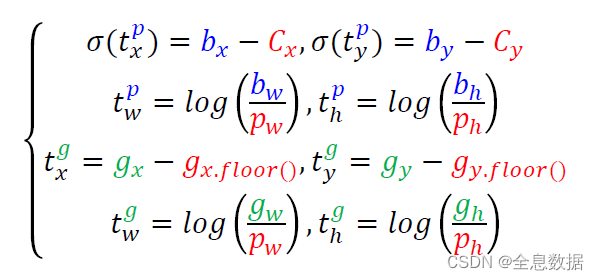
3.1 Yolo层执行解析
黑色:anchor,蓝色:gt,
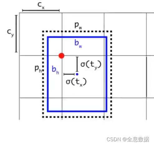
以下代码解析是实现下面的4行公式的:
先对预测的tensor进行维度的调整,原维度为:[b, 3, 85, 13, 13],调整为:[b, 3, 13, 13, 85]
调整维度的作用:为了好计算,
代码为:
prediction = (
            #       b, 3, 85, 13, 13
            x.view(num_samples, self.num_anchors, self.num_classes + 5, grid_size, grid_size)
                #       b, 3, 13, 13, 85, 3:对应3个anchor
                .permute(0, 1, 3, 4, 2)
                .contiguous()  # 作用:经过view、permute之后这些数据在内存里已经碎了,所以用contiguous重新整理一下
        )
然后分别输出预测的x,y,w,h,pred_conf ,pred_cls ,其中x,y,w,h是对应上面4行公式的 σ ( t x p ) \sigma(t^p_x) σ(txp)、 σ ( t y p ) \sigma(t^p_y) σ(typ)、 t w p t^p_w twp、 t h p t^p_h thp,因为预测的x,y是在0-1之间的,所以前面加上sigmoid,pred_conf 是物体的置信度,也在0-1之间,pred_cls 是对每一个的维度进行sigmoid,因此可以进行多类别判断,代码为:
x = torch.sigmoid(prediction[..., 0])  # Center x   # (b,3,13,13)            # 1 +
y = torch.sigmoid(prediction[..., 1])  # Center y   # (b,3,13,13)            # 1 +
w = prediction[..., 2]  # Width                     # (b,3,13,13)            # 1 +
h = prediction[..., 3]  # Height                    # (b,3,13,13)            # 1 +
pred_conf = torch.sigmoid(prediction[..., 4])  # Conf (b,3,13,13)            # 1 + = 5 +
pred_cls = torch.sigmoid(prediction[..., 5:])  # Cls pred. (b,3,13,13,80)    # 80 = 85
因为上面预测输出的x,y,w,h,pred_conf ,pred_cls是基于13×13 cell 的,所以还需要进行下面的计算,代码为:
 def compute_grid_offsets(self, grid_size, cuda=True):
        """ 把初始的anchors根据不同的输出结果的feature-size进行归一化,如根据13*13,return:(a_w/w)*13 """
        # 0<-13; 13<-26; 26<-52
        self.grid_size = grid_size
        g = self.grid_size  # 13, 26, 52
        FloatTensor = torch.cuda.FloatTensor if cuda else torch.FloatTensor
        self.stride = self.img_dim / self.grid_size  # 32, 16, 8 => pixels per grid/feature point represents
        # Calculate offsets for each grid, 因为tensor本身是4维的,所以view成4维
        self.grid_x = torch.arange(g).repeat(g, 1).view([1, 1, g, g]).type(FloatTensor)
        # torch.arange(g): tensor([0,1,2,...,12])
        # torch.arange(g).repeat(g, 1):
        #       tensor([[0,1,2,...,12],
        #               [0,1,2,...,12],
        #               ...
        #               [0,1,2,...,12]])
        #       shape=torch.Size([13, 13])
        # torch.arange(g).repeat(g, 1).view([1, 1, g, g]):
        #       tensor([[[[0,1,2,...,12],
        #                 [0,1,2,...,12],
        #                 ...
        #                 [0,1,2,...,12]]]])
        #       shape=torch.Size([1, 1, 13, 13])
        # todo: 关于 repeat (不是todo,就是为了这个颜色)
        # torch.repeat(m): 在第0维重复m次
        #                  此处如果只用.repeat(g),则会出现[0,1,...,12,0,1,...12,...,0,1,...12]
        # torch.repeat(m, n): 在第0维重复m次,在第1维重复n次

        self.grid_y = torch.arange(g).repeat(g, 1).t().view([1, 1, g, g]).type(FloatTensor)
        # torch.arange(g).repeat(g, 1).t().view([1, 1, g, g]):
        #       tensor([[[[0,0,0,...,0],
        #                 [1,1,1,...,1],
        #                 ...
        #                 [12,12,12,...,12]]]])
        #       shape=torch.Size([1, 1, 13, 13])
        self.scaled_anchors = FloatTensor([(a_w / self.stride, a_h / self.stride) for a_w, a_h in self.anchors])
        # FloatTensor()后会将里面的tuple()变成[]
        # 将anchor变到(0, 13)范围内
        # self.scaled_anchors = tensor([[3.625, 2.8125], [4.875, 6.1875], [11.65625, 10.1875]]) # 3x2
        # self.num_anchors:为了对应(b,3,13,13)中的3,
        self.anchor_w = self.scaled_anchors[:, 0:1].view((1, self.num_anchors, 1, 1))
        # self.scaled_anchors[:, :1]: tensor([[3.625], [4.8750], [11.6562]])
        # self.anchor_w =
        # self.scaled_anchors.view((1, 3, 1, 1)) =
        #                                          tensor([
        #                                                  [
        #                                                    [[3.625]],
        #                                                    [[4.8750]],
        #                                                    [[11.6562]]
        #                                                  ]
        #                                                 ])
        self.anchor_h = self.scaled_anchors[:, 1:2].view((1, self.num_anchors, 1, 1))
然后再把上面计算出的x,y加上cell的序号,把计算出的w,h还原成基于13×13归一化的w,h,代码为:
pred_boxes = FloatTensor(prediction[..., :4].shape)  # (b, 3, 13, 13, 4)
pred_boxes[..., 0] = x.data + self.grid_x
pred_boxes[..., 1] = y.data + self.grid_y
pred_boxes[..., 2] = torch.exp(w.data) * self.anchor_w
pred_boxes[..., 3] = torch.exp(h.data) * self.anchor_h

# 即输出与原图相匹配的bbox
output = torch.cat(
    (  # * stride(=32对于13x13),目的是将(0, 13)的bbox恢复到(0, 416)
        pred_boxes.view(num_samples, -1, 4) * self.stride,
        pred_conf.view(num_samples, -1, 1),
        pred_cls.view(num_samples, -1, self.num_classes),
    ),
    -1,
)
至此,已经实现上面公式中的前两行。
下面来实现上面公式中的后两行,
首先来匹配哪些 anchor 去与 target 对应,那个anchor与target具有最大的IOU,则使用那个anchor来预测物体。
pred_boxes是网络生成预测的tensor,
nB = pred_boxes.size(0)  # batch size, pred_boxes的size: (b, 3, 13, 13, 4)
nA = pred_boxes.size(1)  # anchor size: 3
nC = pred_cls.size(-1)  # class size: 80, pred_cls的size: (b,3,13,13,80)
nG = pred_boxes.size(2)  # grid size: 13
为了使网络生成预测的tensor与target维度相匹配,所以target就使用网络生成预测的tensor的相同的size,
# Output tensors
obj_mask = ByteTensor(nB, nA, nG, nG).fill_(0)  # (b, 3, 13, 13)
noobj_mask = ByteTensor(nB, nA, nG, nG).fill_(1)  # (b, 3, 13, 13)    # mostly candidates are noobj
class_mask = FloatTensor(nB, nA, nG, nG).fill_(0)  # (b, 3, 13, 13)
iou_scores = FloatTensor(nB, nA, nG, nG).fill_(0)  # (b, 3, 13, 13)
tx = FloatTensor(nB, nA, nG, nG).fill_(0)  # (b, 3, 13, 13)
ty = FloatTensor(nB, nA, nG, nG).fill_(0)  # (b, 3, 13, 13)
tw = FloatTensor(nB, nA, nG, nG).fill_(0)  # (b, 3, 13, 13)
th = FloatTensor(nB, nA, nG, nG).fill_(0)  # (b, 3, 13, 13)
tcls = FloatTensor(nB, nA, nG, nG, nC).fill_(0)  # (b, 3, 13, 13, 80)
去挑选使用哪个anchor去预测物体,那个anchor肯定与target物体具有最大的IOU,即target物体与anchor的匹配;
# Convert to position relative to box
#                    高维 低维
target_boxes = target[:, 2:6] * nG  # (0, 1)->(0, 13) (n_boxes, 4)
gxy = target_boxes[:, :2]  # (n_boxes, 2)
gwh = target_boxes[:, 2:]  # (n_boxes, 2)

# anchor如何跟物体对应上
# 此两行的目的:判断哪一个anchor该去预测那一个物体,该物体的bbox具有与anchor最大的IOU
# Get anchors with best iou
# 仅依靠w&h 计算target box和anchor box的交并比, (num_anchor, n_boxes)
ious = torch.stack([bbox_wh_iou(anchor, gwh) for anchor in anchors])
# e.g, 每个anchor都和每个target bbox去算iou,结果存成矩阵(num_anchor, n_boxes)
#                box0    box1    box2    box3    box4    标注框(即label)
# ious=tensor([[0.7874, 0.9385, 0.5149, 0.0614, 0.3477],    anchor0
#              [0.2096, 0.5534, 0.5883, 0.2005, 0.5787],    anchor1
#              [0.8264, 0.6750, 0.4562, 0.2156, 0.7026]])   anchor2
# best_ious:
# tensor([0.8264, 0.9385, 0.5883, 0.2156, 0.7026])
# best_n:
# 属于第几个bbox:0, 1, 2, 3, 4
#       tensor([2, 0, 1, 2, 2])   属于第几个anchor
best_ious, best_n = ious.max(0)  # 最大iou, 与target box交并比最大的anchor的index // [n_boxes], [n_boxes]
# 到目前为止,我们还不知道靠哪一个cell去预测那一个物体,但是我们知道了,无论靠哪一个cell,都应该用那一个anchor去预测
然后再匹配哪个cell去和target物体对应上,首先先得到target物体的gx, gy,再使用 long() 方法得到整数,obj_mask等于1和noobj_mask不等于0的参与后面的计算;
# cell和物体的关系
# Separate target values
# target[:, :2]: (n_boxes, 2) -> img index, class index
# target[].t(): (2, n_boxes) -> b: img index in batch, torch.Size([n_boxes]),
#                               target_labels: class index, torch.Size([n_boxes])
b, target_labels = target[:, :2].long().t()  # long():取整
# gxy.t().shape = shape(gwh.t())=(2, n_boxes)
gx, gy = gxy.t()  # gx = gxy.t()[0], gy = gxy.t()[1]
gw, gh = gwh.t()  # gw = gwh.t()[0], gh = gwh.t()[1]
gi, gj = gxy.long().t()  # .long()去除小数点,找到了具体的cell
# Set masks,这里的b是batch中的第几个
# b:对应着哪张图片
# best_n:对应着哪个anchor
# gj, gi:对应着哪个cell
obj_mask[b, best_n, gj, gi] = 1  # 物体中心点落在的那个cell中的,与target object iou最大的那个3个anchor中的那1个,被设成1
noobj_mask[b, best_n, gj, gi] = 0  # 其相应的noobj_mask被设成0
需要考虑到noobj_mask的best_n,如果3个anchor与target的IOU分别是0.9,0.8,0.7,按照前面的算法,只取0.9的anchor为0,而取0.8,0.7的anchor继续为1,即为背景,这里可能欠考虑,因为其他anchor与target的IOU为0.6的为0,而0.8,0.7的anchor继续为1反而不太合适,所以这里把IOU大于某一个阈值继续取0,
# Set noobj mask to zero where iou exceeds ignore threshold
# ious.t():
# shape: (n_boxes, num_anchor)
# i: box id
# b[i]: img index in that batch
# E.g 假设有4个boxes,其所属图片在batch中的index为[0, 0, 1, 2], 即前2个boxes都属于本batch中的第0张图
#     则b[0] = b[1] = 0 都应所属图片在batch中的index,即batch中的第几张图
for i, anchor_ious in enumerate(ious.t()):
    # 如果anchor_iou>ignore_thres,则即使它不是obj(非best_n),同样不算noobj
    noobj_mask[b[i], anchor_ious > ignore_thres, gj[i], gi[i]] = 0
# box: 3 anchor
# IOU:0.9 0.85 0.8 --> om: 1 0 0
#                  --> nm: 0 0 0
# 工作中常用: FaceBoxes(SSD): github:bipartite machining + ohem (online hard example mining) 先训练loss比较大的
因此我们得到4行公式的后2行,以及类别的tensor
# Coordinates
tx[b, best_n, gj, gi] = gx - gx.floor()  # x_offset (0, 1)
ty[b, best_n, gj, gi] = gy - gy.floor()  # y_offset (0, 1)
# Width and height
tw[b, best_n, gj, gi] = torch.log(gw / anchors[best_n][:, 0] + 1e-16)
th[b, best_n, gj, gi] = torch.log(gh / anchors[best_n][:, 1] + 1e-16)
# One-hot encoding of label
tcls[b, best_n, gj, gi, target_labels] = 1
3.2 Loss的组成
回归的loss是上面4行公式的 t p t^p tp与 t g t^g tg的回归,使用的mse Loss,
conf的loss使用的是bce Loss,
类别也是使用的是bce Loss,
# Loss : Mask outputs to ignore non-existing objects (except with conf. loss)
# 可以看到,真正参与loss计算的,仍然是·与t·,即offset regress
# Reg Loss
loss_x = self.mse_loss(x[obj_mask], tx[obj_mask])  # mse_loss:就是L2 loss
loss_y = self.mse_loss(y[obj_mask], ty[obj_mask])
loss_w = self.mse_loss(w[obj_mask], tw[obj_mask])
loss_h = self.mse_loss(h[obj_mask], th[obj_mask])

# Conf Loss
# 因为这里conf选择的是bce_loss,因为对于noobj,基本都能预测对,所以loss_conf_noobj通常比较小
# 所以此时为了平衡,noobj_scale往往大于obj_scale, (100, 1),本质平衡loss
# 实际上,这里的conf loss就是做了个0-1分类,0就是noobj, 1就是obj
loss_conf_obj = self.bce_loss(pred_conf[obj_mask], tconf[obj_mask])
loss_conf_noobj = self.bce_loss(pred_conf[noobj_mask], tconf[noobj_mask])
loss_conf = self.obj_scale * loss_conf_obj + self.noobj_scale * loss_conf_noobj

# Class Loss
loss_cls = self.bce_loss(pred_cls[obj_mask], tcls[obj_mask])

# Total Loss
total_loss = loss_x + loss_y + loss_w + loss_h + loss_conf + loss_cls
然后可以使用SGBM优化器或adam优化器进行bp就可以训练啦。


 394
394


 被折叠的 条评论
为什么被折叠?
被折叠的 条评论
为什么被折叠?
 到【灌水乐园】发言


