UFIDL稀疏自编码代码实现及解释

UFIDL稀疏自编码代码实现及解释

1.今天我们来讲一下UFIDL的第一个练习。

1.我们来看看最难的一个.m文件

%% ---------- YOUR CODE HERE --------------------------------------
%  Instructions: Compute the cost/optimization objective J_sparse(W,b) for the Sparse Autoencoder,
%                and the corresponding gradients W1grad, W2grad, b1grad, b2grad.
%
% W1grad, W2grad, b1grad and b2grad should be computed using backpropagation.
% Note that W1grad has the same dimensions as W1, b1grad has the same dimensions
% as b1, etc.  Your code should set W1grad to be the partial derivative of J_sparse(W,b) with
% respect to W1.  I.e., W1grad(i,j) should be the partial derivative of J_sparse(W,b) 
% with respect to the input parameter W1(i,j).  Thus, W1grad should be equal to the term 
% [(1/m) \Delta W^{(1)} + \lambda W^{(1)}] in the last block of pseudo-code in Section 2.2 
% of the lecture notes (and similarly for W2grad, b1grad, b2grad).
% 
% Stated differently, if we were using batch gradient descent to optimize the parameters,
% the gradient descent update to W1 would be W1 := W1 - alpha * W1grad, and similarly for W2, b1, b2. 
% 
% size(data, 1) % 64
% size(W1)   % 25 64
% size(W2)   % 64 25
% size(b1)   % 25  1
% size(b2)   % 64  1


%样本的个数
m = size(data, 2);


%前向传播
%第二层的输入值
z_2 = W1 * data + repmat(b1, 1, m);
%第二层的激活值
a_2 = sigmoid(z_2); % 25 10000


%计算rho_hat的值，其值为第二层的每个维度(64)上的平均激活度,sum(a_2,2)表示对第二维求和，即对每一行求和
rho_hat = sum(a_2, 2) / m; % This doesn't contain an x because the data
                       % above "has" the x
%第三层的输入
z_3 = W2 * a_2 + repmat(b2, 1, m);
%第三层的激活
a_3 = sigmoid(z_3); % 64 10000


%激活值与实际值的差
diff = a_3 - data;


%稀疏自编码的惩罚，KLdivergence(相对熵)
sparse_penalty = kl(sparsityParam, rho_hat);

%简化的代价函数
%这个写的比较简洁
J_simple = sum(sum(diff.^2)) / (2*m);


%正则项，即所有W元素的平方和
%这个写得也不错，W1(:)使得矩阵的元素按列重新排布
reg = sum(W1(:).^2) + sum(W2(:).^2);


%总的代价
cost = J_simple + beta * sparse_penalty + lambda * reg / 2;


% Backpropogation

delta_3 = diff .*            (a_3 .* (1-a_3));   % 64 10000


%计算残差2的基本部分
d2_simple = W2' * delta_3;   % 25 10000
%计算残差2的惩罚
d2_pen = kl_delta(sparsityParam, rho_hat);


%计算残差2
delta_2 = (d2_simple + beta * repmat(d2_pen,1, m)) .* a_2 .* (1-a_2);


%计算b的梯度
b2grad = sum(delta_3, 2)/m;
b1grad = sum(delta_2, 2)/m;


%计算W的梯度
W2grad = delta_3 * a_2'/m  + lambda * W2; % 25 64
W1grad = delta_2 * data'/m + lambda * W1; % 25 64


%-------------------------------------------------------------------
% After computing the cost and gradient, we will convert the gradients back
% to a vector format (suitable for minFunc).  Specifically, we will unroll
% your gradient matrices into a vector.


grad = [W1grad(:) ; W2grad(:) ; b1grad(:) ; b2grad(:)];


end


%-------------------------------------------------------------------
% Here's an implementation of the sigmoid function, which you may find useful
% in your computation of the costs and the gradients.  This inputs a (row or
% column) vector (say (z1, z2, z3)) and returns (f(z1), f(z2), f(z3)). 


function sigm = sigmoid(x)
  sigm = 1 ./ (1 + exp(-x));
end


%相对熵
function ans = kl(r, rh)
  ans = sum(r .* log(r ./ rh) + (1-r) .* log( (1-r) ./ (1-rh)));
end


%相对熵的残差计算公式
function ans = kl_delta(r, rh)
  ans = -(r./rh) + (1-r) ./ (1-rh);
end


%sigmoid函数的导数
function pr = prime(x)
    pr = sigmoid(x) .* (1 - sigmoid(x));
end

我对上述进行了解释。

接下去是SampleIMAGES文件，这个比较简单我就不解释了

function patches = sampleIMAGES()
% sampleIMAGES
% Returns 10000 patches for training

load IMAGES;    % load images from disk 

patchsize = 8;  % we'll use 8x8 patches 
numpatches = 10000;

% Initialize patches with zeros.  Your code will fill in this matrix--one
% column per patch, 10000 columns. 
patches = zeros(patchsize*patchsize, numpatches);

%% ---------- YOUR CODE HERE --------------------------------------
%  Instructions: Fill in the variable called "patches" using data 
%  from IMAGES.  
%  
%  IMAGES is a 3D array containing 10 images
%  For instance, IMAGES(:,:,6) is a 512x512 array containing the 6th image,
%  and you can type "imagesc(IMAGES(:,:,6)), colormap gray;" to visualize
%  it. (The contrast on these images look a bit off because they have
%  been preprocessed using using "whitening."  See the lecture notes for
%  more details.) As a second example, IMAGES(21:30,21:30,1) is an image
%  patch corresponding to the pixels in the block (21,21) to (30,30) of
%  Image 1


% imagesc(IMAGES(:,:,10)) % 1-10
% size(patches)      % 64 x 10000
% size(patches(:,1)) % 64 x 1

for i = 1:numpatches
    x = randi(512-8+1);
    y = randi(512-8+1);
    sample = IMAGES(x:x+7,y:y+7,randi(10));
    patches(:,i) = sample(:);
end

%% ---------------------------------------------------------------
% For the autoencoder to work well we need to normalize the data
% Specifically, since the output of the network is bounded between [0,1]
% (due to the sigmoid activation function), we have to make sure 
% the range of pixel values is also bounded between [0,1]
patches = normalizeData(patches);

end


%% ---------------------------------------------------------------
function patches = normalizeData(patches)

% Squash data to [0.1, 0.9] since we use sigmoid as the activation
% function in the output layer

% Remove DC (mean of images). 
patches = bsxfun(@minus, patches, mean(patches));

% Truncate to +/-3 standard deviations and scale to -1 to 1
pstd = 3 * std(patches(:));
patches = max(min(patches, pstd), -pstd) / pstd;

% Rescale from [-1,1] to [0.1,0.9]
patches = (patches + 1) * 0.4 + 0.1;

end

从10幅图像里面随机抽取10000个图像块，并进行了一些归一化处理。

接下去是计算梯度函数

function numgrad = computeNumericalGradient(J, theta)
% numgrad = computeNumericalGradient(J, theta)
% theta: a vector of parameters
% J: a function that outputs a real-number. Calling y = J(theta) will return the
% function value at theta. 
  
% Initialize numgrad with zeros
numgrad = zeros(size(theta));


%% ---------- YOUR CODE HERE --------------------------------------
% Instructions: 
% Implement numerical gradient checking, and return the result in numgrad.  
% (See Section 2.3 of the lecture notes.)
% You should write code so that numgrad(i) is (the numerical approximation to) the 
% partial derivative of J with respect to the i-th input argument, evaluated at theta.  
% I.e., numgrad(i) should be the (approximately) the partial derivative of J with 
% respect to theta(i).
%                
% Hint: You will probably want to compute the elements of numgrad one at a time. 


% size(theta)   2 1 | 3289 1
% size(numgrad) 2 1 | 3289 1
eps = 1e-4;
n = size(numgrad);
I = eye(n, n);
for i = 1:size(numgrad)
    %通过单位矩阵来构造向量，比较有趣
    eps_vec = I(:,i) * eps;
    numgrad(i) = (J(theta + eps_vec) - J(theta - eps_vec)) / (2 * eps);
end


% numgrad = (J(theta + eps) - J(theta - eps)) / (2 * eps)








%% ---------------------------------------------------------------
end

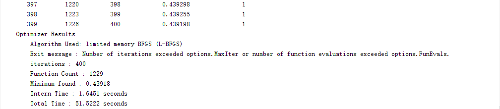
最后我们运行官方的train文件，并等待结果(大约1分钟左右)

我们可以看到matlab的输出

可以看到我们我们通过BFGS(共轭梯度下降法)，总共迭代了400次，花了51秒。

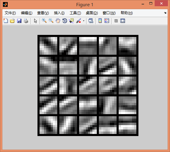
下面是稀疏自编码的结果