对数几率回归Logistic Regression（Matlab）

这里的数据均来源于吴恩达老师机器学习的课程。

       上一篇内容是线性回归，利用线性模型进行回归学习，最终结果是找到一组合适的theta值，使代价函数的值最小，可是对于分类任务该如何解决呢？其实也是希望学习到的也是一组满足这种条件的theta。

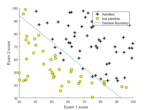
       先从简单的二分类问题考虑，比如从两门考试的成绩x1,x2，判断录取与否。对于结果y只有两种取值，,录取时y=1,不录取y=0.这时候，如果还像之前那怎样直接相乘算出预测值就不太合适了，因为此时需要把预测值的范围控制在[0,1],想要做到这一点，可以利用sigmoid函数，对数几率函数(logistic function)是sigmoid函数的重要代表。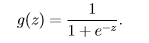也就是说，要找到一组theta，在预测函数是这个样子的条件下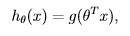，代价函数值最小。

      总的来说，方法没有变，只是改了预测函数的形式。

二分类

[plain]  view plain  copy

1. data = load('ex2data1.txt');  
2. X = data(:, [1, 2]); y = data(:, 3);  
3. figure; hold on;  
4. pos=find(y==1);  
5. neg=find(y==0);  
6. plot(X(pos,1),X(pos,2),'k+','LineWidth',2,'MarkerSize',7);  
7. plot(X(neg,1),X(neg,2),'ko','MarkerFaceColor','y','MarkerSize',7);  
8. % Labels and Legend  
9. xlabel('Exam 1 score')  
10. ylabel('Exam 2 score')  
11. hold off;  
12. [m, n] = size(X);  
13. % Add intercept term to x and X_test  
14. X = [ones(m, 1) X];  
15. % Initialize fitting parameters  
16. initial_theta = zeros(n + 1, 1);  
17. options = optimset('GradObj', 'on', 'MaxIter', 400);  
18. [theta, cost] = fminunc(@(t)(costFunction(t, X, y)), initial_theta, options);  
19. %plot decision boundary  
20. hold on;  
21. if size(X, 2) <= 3  
22.     % Only need 2 points to define a line, so choose two endpoints  
23.     plot_x = [min(X(:,2))-2,  max(X(:,2))+2];  
24.     % Calculate the decision boundary line  
25.     plot_y = (-1./theta(3)).*(theta(2).*plot_x + theta(1));  
26.     plot(plot_x, plot_y)  
27.     % Legend, specific for the exercise  
28.     legend('Admitted', 'Not admitted', 'Decision Boundary')  
29.     axis([30, 100, 30, 100])  
30. else  
31.     % Here is the grid range  
32.     u = linspace(-1, 1.5, 50);  
33.     v = linspace(-1, 1.5, 50);  
34.     z = zeros(length(u), length(v));  
35.     % Evaluate z = theta*x over the grid  
36.     for i = 1:length(u)  
37.         for j = 1:length(v)  
38.             z(i,j) = mapFeature(u(i), v(j))*theta;  
39.         end  
40.     end  
41.     z = z';   
42.     contour(u, v, z, [0, 0], 'LineWidth', 2)  
43. end  
44. hold off;  

[plain]  view plain  copy

1. %costFunction.m  
2. function [J, grad] = costFunction(theta, X, y)  
3. m = length(y); % number of training examples  
4. J = 0;  
5. grad = zeros(size(theta));  
6. h=1.0./(1.0+exp(-1*X*theta));  
7. m=size(y,1);  
8. J=((-1*y)'*log(h)-(1-y)'*log(1-h))/m;  
9. for i=1:size(theta,1),  
10.     grad(i)=((h-y)'*X(:,i))/m;  
11. end  
12. end  

二分类的决策边界不总是直线的，这取决于你的假设函数。例如，当给出的训练数据是这样的：

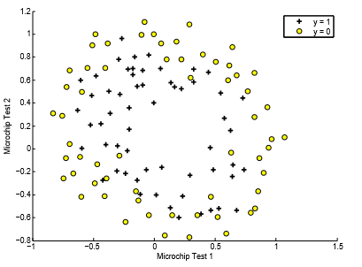
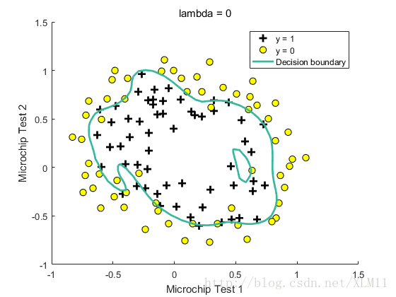
简单的特征x1,x2,就不能满足了，需要做个映射。

这样就可以很好的分类了。

多分类

二分类问题也可以推广到多分类问题，例如有A，B，C三类，可以训练出三组theta，对于theta1，训练数据的结果只有1-->A，0-->B,C,y预测结果也是[0,1],theta2,theta3,也是如此,最终判断归于是哪一类，就取这三个预测结果更大的那一类。就不累述了。