空间转录组 DeepST 2

qq_27648263

已于 2022-10-15 21:53:23 修改

阅读量1.1k

点赞数 4

文章标签： python 深度学习机器学习

于 2022-10-15 20:42:17 首次发布

本文链接：https://blog.csdn.net/qq_27648263/article/details/127316497

版权

DeepST共三项工作，聚类分析、单细胞和空间转录组数据联合分析（解卷积）、空间对齐。第一项任务已经看完代码了，现在看第二项联合分析。

此项以人类淋巴结Human_Lymph_Node数据为例（10X），作者已经处理好数据，并上传到谷歌云盘上了，直接下载用就好了。

原始数据如下。

https://support.10xgenomics.com/spatial-gene-expression/datasets/1.0.0/V1_Human_Lymph_Node

下面还是看代码。

import scanpy as sc
from DeepST import DeepST
dataset = 'Human_Lymph_Node'
file_path = 'Human_Lymph_Node/' 
# set random seed
random_seed = 50
DeepST.fix_seed(random_seed)
# read ST data
adata = sc.read_h5ad(file_path+'ST.h5ad')
adata.var_names_make_unique()

# preprocessing for ST data
DeepST.preprocess(adata)

# build graph
DeepST.construct_interaction(adata)
DeepST.add_contrastive_label(adata)

# read scRNA daa
adata_sc = sc.read(file_path+'scRNA.h5ad')
adata_sc.var_names_make_unique()

# preprocessing for scRNA data
DeepST.preprocess(adata_sc)

以上主函数，直到这里，都没有新的代码，具体可看上一篇博客。具体包括数据预处理，构建正负类标签、邻接矩阵等。

然后挑选单细胞数据和空间转录组数据的共同基因。

def filter_with_overlap_gene(adata, adata_sc):
    # remove all-zero-valued genes
    #sc.pp.filter_genes(adata, min_cells=1)
    #sc.pp.filter_genes(adata_sc, min_cells=1)
    
    if 'highly_variable' not in adata.var.keys():
       raise ValueError("'highly_variable' are not existed in adata!")
    else:    
       adata = adata[:, adata.var['highly_variable']]
       
    if 'highly_variable' not in adata_sc.var.keys():
       raise ValueError("'highly_variable' are not existed in adata_sc!")
    else:    
       adata_sc = adata_sc[:, adata_sc.var['highly_variable']]   

    # Refine `marker_genes` so that they are shared by both adatas
    genes = list(set(adata.var.index) & set(adata_sc.var.index))
    genes.sort()
    print('Number of overlap genes:', len(genes))

    adata.uns["overlap_genes"] = genes
    adata_sc.uns["overlap_genes"] = genes
    
    adata = adata[:, genes]
    adata_sc = adata_sc[:, genes]
    
    return adata, adata_sc

分别筛选单细胞核空转的高表达基因，然后挑选共同的基因。

继续，构建正负类特征，这个也已介绍。

DeepST.get_feature(adata)

继而，构建模型。

model = DeepST.Train(adata, adata_sc, epochs=1200, deconvolution=True)

这里解卷积就是为真了，并且epochs变大了，模型结构与之前一致，这里就不赘述了。

初始化程序不放上了，用到的时候会再说。

判断解卷积，在缺失值位置10X数据正负类赋值为0.

if self.deconvolution:
   self.adata_sc = adata_sc.copy() 
    
   if isinstance(self.adata.X, csc_matrix) or isinstance(self.adata.X, csr_matrix):
      self.feat_sp = adata.X.toarray()[:, ]
   else:
      self.feat_sp = adata.X[:, ]
   if isinstance(self.adata_sc.X, csc_matrix) or isinstance(self.adata_sc.X, csr_matrix):
      self.feat_sc = self.adata_sc.X.toarray()[:, ]
   else:
      self.feat_sc = self.adata_sc.X[:, ]
    
   # fill nan as 0
   self.feat_sc = pd.DataFrame(self.feat_sc).fillna(0).values
   self.feat_sp = pd.DataFrame(self.feat_sp).fillna(0).values
  
   self.feat_sc = torch.FloatTensor(self.feat_sc).to(self.device)
   self.feat_sp = torch.FloatTensor(self.feat_sp).to(self.device)

   if self.adata_sc is not None:
      self.dim_input = self.feat_sc.shape[1] 

   self.n_cell = adata_sc.n_obs
   self.n_spot = adata.n_obs

仔细看下模型训练，这个和之前有不少不同的。

adata, adata_sc = model.train_map()

首先是训练空间转录组的模型，然后提取特征，这个和之前的没有任何区别，不做介绍了。

emb_sp = self.train()

然后训练单细胞数据的模型

emb_sc = self.train_sc()

首先构建编码器，这里选取的是六层线性层编码器（三层编码，三层解码），输出是重构的单细胞数据（输入输出维度相同，这个和空转是一样的）。

class Encoder_sc(torch.nn.Module):
    def __init__(self, dim_input, dim_output, dropout=0.0, act=F.relu):
        super(Encoder_sc, self).__init__()
        self.dim_input = dim_input
        self.dim1 = 256
        self.dim2 = 64
        self.dim3 = 32
        self.act = act
        self.dropout = dropout
        
        #self.linear1 = torch.nn.Linear(self.dim_input, self.dim_output)
        #self.linear2 = torch.nn.Linear(self.dim_output, self.dim_input)
        
        #self.weight1_en = Parameter(torch.FloatTensor(self.dim_input, self.dim_output))
        #self.weight1_de = Parameter(torch.FloatTensor(self.dim_output, self.dim_input))
        
        self.weight1_en = Parameter(torch.FloatTensor(self.dim_input, self.dim1))
        self.weight2_en = Parameter(torch.FloatTensor(self.dim1, self.dim2))
        self.weight3_en = Parameter(torch.FloatTensor(self.dim2, self.dim3))
        
        self.weight1_de = Parameter(torch.FloatTensor(self.dim3, self.dim2))
        self.weight2_de = Parameter(torch.FloatTensor(self.dim2, self.dim1))
        self.weight3_de = Parameter(torch.FloatTensor(self.dim1, self.dim_input))
      
        self.reset_parameters()

    def reset_parameters(self):
        torch.nn.init.xavier_uniform_(self.weight1_en)
        torch.nn.init.xavier_uniform_(self.weight1_de)
        
        torch.nn.init.xavier_uniform_(self.weight2_en)
        torch.nn.init.xavier_uniform_(self.weight2_de)
        
        torch.nn.init.xavier_uniform_(self.weight3_en)
        torch.nn.init.xavier_uniform_(self.weight3_de)
        
    def forward(self, x):
        x = F.dropout(x, self.dropout, self.training)
        
        #x = self.linear1(x)
        #x = self.linear2(x)
        
        #x = torch.mm(x, self.weight1_en)
        #x = torch.mm(x, self.weight1_de)
        
        x = torch.mm(x, self.weight1_en)
        x = torch.mm(x, self.weight2_en)
        x = torch.mm(x, self.weight3_en)
        
        x = torch.mm(x, self.weight1_de)
        x = torch.mm(x, self.weight2_de)
        x = torch.mm(x, self.weight3_de)
        
        return x

然后是训练模型，损失函数就是输入和输出的MSE。

def train_sc(self):
    self.model_sc = Encoder_sc(self.dim_input, self.dim_output).to(self.device)
    self.optimizer_sc = torch.optim.Adam(self.model_sc.parameters(), lr=self.learning_rate_sc)  
    
    print('Begin to train scRNA data...')
    for epoch in tqdm(range(self.epochs)):
        self.model_sc.train()
        
        emb = self.model_sc(self.feat_sc)
        loss = F.mse_loss(emb, self.feat_sc)
        
        self.optimizer_sc.zero_grad()
        loss.backward()
        self.optimizer_sc.step()
        
    print("Optimization finished for cell representation learning!")
    
    with torch.no_grad():
        self.model_sc.eval()
        emb_sc = self.model_sc(self.feat_sc)
     
        return emb_sc

随后将单细胞数据和空转数据数据正则化一下，构建映射模型。

self.adata.obsm['emb_sp'] = emb_sp.detach().cpu().numpy()
self.adata_sc.obsm['emb_sc'] = emb_sc.detach().cpu().numpy()

# Normalize features for consistence between ST and scRNA-seq
emb_sp = F.normalize(emb_sp, p=2, eps=1e-12, dim=1)
emb_sc = F.normalize(emb_sc, p=2, eps=1e-12, dim=1)

self.model_map = Encoder_map(self.n_cell, self.n_spot).to(self.device)  
  
self.optimizer_map = torch.optim.Adam(self.model_map.parameters(), lr=self.learning_rate, weight_decay=self.weight_decay)

再来看Encoder_map模型结构，传入的参数分别是单细胞数据细胞个数和空转数据spot个数（以这两个参数为行和列构建了一个矩阵为映射矩阵，最终也是要训练得到映射矩阵）。

class Encoder_map(torch.nn.Module):
    def __init__(self, n_cell, n_spot):
        super(Encoder_map, self).__init__()
        self.n_cell = n_cell
        self.n_spot = n_spot
          
        self.M = Parameter(torch.FloatTensor(self.n_cell, self.n_spot))
        self.reset_parameters()

    def reset_parameters(self):
        torch.nn.init.xavier_uniform_(self.M)
        
    def forward(self):
        x = self.M
        
        return x

再来看映射训练，生成M矩阵，计算损失函数，优化参数。

        for epoch in tqdm(range(self.epochs)):
            self.model_map.train()
            self.map_matrix = self.model_map()
        
            loss_recon, loss_NCE = self.loss(emb_sp, emb_sc)
             
            loss = self.lamda1*loss_recon + self.lamda2*loss_NCE 
        
            self.optimizer_map.zero_grad()
            loss.backward()
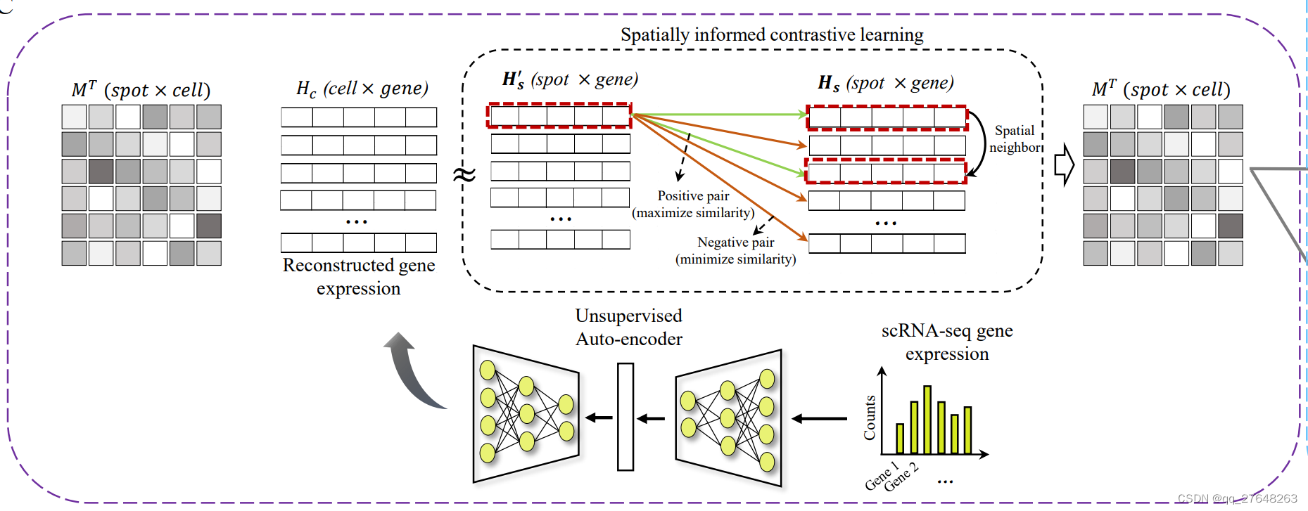
            self.optimizer_map.step()

具体来看损失函数。损失函数包括两部分，重构损失和对比损失（不太确定这么形容对不对）。首先由M经过softmax后得到map_probs，转置后与单细胞编码数据相乘即为重构空间转录组数据。

def loss(self, emb_sp, emb_sc):
    '''\
    Calculate loss

    Parameters
    ----------
    emb_sp : torch tensor
        Spatial spot representation matrix.
    emb_sc : torch tensor
        scRNA cell representation matrix.

    Returns
    -------
    Loss values.

    '''
    # cell-to-spot
    map_probs = F.softmax(self.map_matrix, dim=1)   # dim=0: normalization by cell
    self.pred_sp = torch.matmul(map_probs.t(), emb_sc)
       
    loss_recon = F.mse_loss(self.pred_sp, emb_sp, reduction='mean')
    loss_NCE = self.Noise_Cross_Entropy(self.pred_sp, emb_sp)
       
    return loss_recon, loss_NCE

重构的空间转录组数据与原始的空间转录组编码数据的MSE值即为重构损失。对比损失这一部分可以参照SimCLR模型，即相近的越相似越好，不相近的越不相似越好，这里的相近指的空间相近，相似指的余弦相似度。具体来说，每一个spot和其邻接矩阵中有连接的spot为正类，其他spot为负类，这个方法最初在陈洛南的stMVC中图像特征提取中见到过。

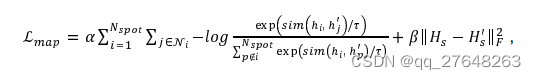
具体来看下对比损失函数，余弦相似度的程序不放进去了。

计算分母的时候（k），是不是应该是

k=torch.exp(mat-torch.diag_embed(torch.diag(a, 0))).sum(axis=1)

其他的都是按照公式计算的，请路过大佬指教。

    def Noise_Cross_Entropy(self, pred_sp, emb_sp):
        '''\
        Calculate noise cross entropy. Considering spatial neighbors as positive pairs for each spot
            
        Parameters
        ----------
        pred_sp : torch tensor
            Predicted spatial gene expression matrix.
        emb_sp : torch tensor
            Reconstructed spatial gene expression matrix.
    
        Returns
        -------
        loss : float
            Loss value.
    
        '''
        
        mat = self.cosine_similarity(pred_sp, emb_sp) 
        k = torch.exp(mat).sum(axis=1) - torch.exp(torch.diag(mat, 0))
        
        # positive pairs
        p = torch.exp(mat)
        p = torch.mul(p, self.graph_neigh).sum(axis=1)
        
        ave = torch.div(p, k)
        loss = - torch.log(ave).mean()
        
        return loss

这样，经过三次训练，就得到了空转编码数据，单细胞编码数据，映射矩阵。

        with torch.no_grad():
            self.model_map.eval()
            emb_sp = emb_sp.cpu().numpy()
            emb_sc = emb_sc.cpu().numpy()
            map_matrix = F.softmax(self.map_matrix, dim=1).cpu().numpy() # dim=1: normalization by cell
            
            self.adata.obsm['emb_sp'] = emb_sp
            self.adata_sc.obsm['emb_sc'] = emb_sc
            self.adata.obsm['map_matrix'] = map_matrix.T # spot x cell

            return self.adata, self.adata_sc

继续，做单细胞和空转数据映射。

from DeepST.utils import project_cell_to_spot
project_cell_to_spot(adata, adata_sc, retain_percent=0.15)

具体来看程序。

1.只保留映射矩阵前百分之十的值，其他值置零。

2.根据单细胞数据的标签，构建单细胞类型矩阵。

3.映射矩阵乘单细胞标签矩阵即空转标签矩阵。

4.空转标签矩阵正则化。

def project_cell_to_spot(adata, adata_sc, retain_percent=0.1):
    '''\
    Project cell types onto ST data using mapped matrix in adata.obsm

    Parameters
    ----------
    adata : anndata
        AnnData object of spatial data.
    adata_sc : anndata
        AnnData object of scRNA-seq reference data.
    retrain_percent: float    
        The percentage of cells to retain. The default is 0.1.
    Returns
    -------
    None.

    '''
    
    # read map matrix 
    map_matrix = adata.obsm['map_matrix']   # spot x cell
   
    # extract top-k values for each spot
    map_matrix = extract_top_value(map_matrix,retain_percent) # filtering by spot
    
    # construct cell type matrix
    matrix_cell_type = construct_cell_type_matrix(adata_sc)
    matrix_cell_type = matrix_cell_type.values
       
    # projection by spot-level
    matrix_projection = map_matrix.dot(matrix_cell_type)
   
    # rename cell types
    cell_type = list(adata_sc.obs['cell_type'].unique())
    cell_type = [str(s) for s in cell_type]
    cell_type.sort()
    #cell_type = [s.replace(' ', '_') for s in cell_type]
    df_projection = pd.DataFrame(matrix_projection, index=adata.obs_names, columns=cell_type)  # spot x cell type
    
    #normalize by row (spot)
    df_projection = df_projection.div(df_projection.sum(axis=1), axis=0).fillna(0)

    #add projection results to adata
    adata.obs[df_projection.columns] = df_projection

最后进行可视化。

# Visualization of spatial distribution of scRNA-seq data
import matplotlib as mpl
with mpl.rc_context({'axes.facecolor':  'black',
                     'figure.figsize': [4.5, 5]}):

         sc.pl.spatial(adata, cmap='magma',
                  # selected cell types
                  color=['B_Cycling', 'B_GC_LZ', 'B_GC_DZ', 'B_GC_prePB'],
                  ncols=4, size=1.3,
                  img_key='hires',
                  # limit color scale at 99.2% quantile of cell abundance
                  vmin=0, vmax='p99.2'
                 )