Gaussian Process(高斯过程) GPSS暑校笔记总计Ⅱ（英文版）——高斯过程介绍二

Stochastic Process

a stochastic process is a collection of random variable indexed by some variable $x\in \mathcal{X}$.
$$f=\left\{\begin{array}{c}f(x):x\in \mathcal{X}\end{array}\right\}$$
$f$ can be thought of as a function of location $x$.

$f$ is an infinite dimensional process. However, thankfully we only need consider the finite dimensional distributions (FDDs), i.e., for all $x_1,...x_n$ and for all $n\in N$
$P(f(x_1)\le y_1,...,f(x_n)\le y_n)$
as these uniquely determine the law of $f$ .

A Gaussian process is a stochastic process with Gaussian FDDs, i.e.
$(f(x_1)...f(x_n))\sim \mathcal{N}(\mu ,\Sigma )$

Import properties

• Property 1: $x\sim \mathcal{N}(\mu ,\Sigma )$ if and only if $AX\sim {\mathcal{N}}_p(A\mu ,A\Sigma A^T)$
  So, sum of Gaussian is Gaussian (taking $A$ as ones vector), and marginal distributions of multivariate are still Gaussian. (taking $A$ is a vector with [0 0 0 1])
• Property 2: Conditional distributions are still Gaussian.

Suppose:
$$X=\left(\begin{array}{c}{X}_1\\ X_2\end{array}\right)\sim \mathcal{N}(\mu ,\Sigma )$$
where,
$$\mu =\left(\begin{array}{c}{\mu }_1\\ {\mu }_2\end{array}\right)$$

$$\Sigma =\left(\begin{array}{cc}{\Sigma }_{11}& {\Sigma }_{12}\\ {\Sigma }_{21}& {\Sigma }_{22}\end{array}\right)$$

Then when we only observe only the part of the result, here $X_1$:
$$(X_2|X_1=x_1)\sim \mathcal{N}({\mu }_2+{\Sigma }_{21}{\Sigma }_{11}^{-1}(x_1-{\mu }_1),{\Sigma }_{22}-{\Sigma }_{21}{\Sigma }_{11}^{-1}{\Sigma }_{12})$$

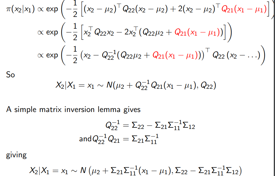
$$\begin{array}{rl}\pi \left(x_2|x_1\right)& =\frac{\pi \left(x_1,x_2\right)}{\pi \left(x_1\right)}\propto \pi \left(x_1,x_2\right)\\ & \propto \exp \left(-\frac{1}{2}(x-\mu {)}^{\top }{\Sigma }^{-1}(x-\mu )\right)\\ & \propto \exp \left(-\frac{1}{2}\left[{\left(x_2-{\mu }_2\right)}^{\top }{Q}_{22}\left(x_2-{\mu }_2\right)+2{\left(x_2-{\mu }_2\right)}^{\top }{Q}_{21}\left(x_1-{\mu }_1\right)\right]\right)\\ & \propto \exp \left(-\frac{1}{2}\left[{\left(x_2-{\mu }_2\right)}^{\top }{Q}_{22}\left(x_2-{\mu }_2\right)+2{\left(x_2-{\mu }_2\right)}^{\top }{Q}_{21}\left(x_1-{\mu }_1\right)\right]\right)\\ \text{ So }{X}_2|X_1=x_1\text{ is Gaussian. }& \end{array}$$

Conditional Update of GP

So suppose $f$ is a Gaussian Process, then,
$$f(x_1),f(x_2)...f(x_n),f(x)\sim \mathcal{N}(\mu ,\Sigma )$$
if we observe its value at $x_1,...,x_n$, then
$$f(x)|f(x_1)...f(x_n)\sim \mathcal{N}({\mu }^{\ast },{\sigma }^{\ast })$$

Why we use GP

1. The GP class of models is closed under various operations.
2. non-parametric/kernel regression
3. Naturalness of GP Framework
4. Uncertainty estimates from emulators

Why GPs: Closed under various operations

• Closed under addition
  $f1(\cdot ),f2(\cdot )\sim GP$ then $(f1+f2)(\cdot )\sim GP$
• Closed under Bayesian conditioning, i.e., if we observe
  $$D=(f(x1),...,f(xn))$$
  then
  $$(f|D)\sim GP$$
• Closed under any linear operation. If $f\sim GP(m(\cdot ),k(\cdot ,\cdot ))$, then if $L$ is a linear operator
  $$L◦f\sim GP(L◦m,L^2◦k)$$

Why GPs: Non-Parametric Regression

Suppose that we are given data
$$(x_i,y_i{)}_{i=1}^n$$
Linear Regression
$$y=x^T\beta +ϵ$$
can be written in form of inner products
$$x^{T}x$$

$$\begin{gathered} \hat{\beta }=argmin||y-X\beta |{|}_2^2+{\sigma }^2||\beta |{|}^2 \\ \hat{\beta }=(X^{T}X+{\Sigma }^{2}I{)}^{-1}{X}^{T}y \\ \hat{\beta }=X^T(X{X}^T+{\sigma }^{2}I{)}^{-1}y(thedualform) \end{gathered}$$

At first, the dual form looks like we’ve made the problem harder:
$$
XX^T ;is ;n*n \

X^TX; is ; p*p
$$
but the dual form makes clear that linear regression only uses inner products.

The best prediction of $y$ at a new location $x^{{}^{\prime }}$ is:
$$\begin{gathered} \hat{y}=x^{{}^{\prime }T}\hat{\beta } \\ \hat{y}=x^{{}^{\prime }T}{X}^T(X{X}^T+{\sigma }^{2}I{)}^{-1}y \\ \hat{y}=k(x^{{}^{\prime }})(K+{\sigma }^{2}I{)}^{-1}y \end{gathered}$$
where,
$$k(x^{{}^{\prime }}):=(x^{{}^{\prime }}{x}_1,...,x^{{}^{\prime }}{x}_n)$$
and
$$K_{ij}:=x_i^T{x}_j$$
these are kernel matrices, every element is the inner product between two rows of training points. And note the similarity to the GP conditional mean we derived before. If:
$$\left(\begin{array}{c}{y}_1\\ y_2\end{array}\right)\sim \mathcal{N}\left(\begin{array}{cc}0,& \left(\begin{array}{cc}{\Sigma }_{11}& {\Sigma }_{12}\\ {\Sigma }_{21}& {\Sigma }_{22}\end{array}\right)\end{array}\right)$$
then,
$$E(y^{{}^{\prime }}|y)={\Sigma }_{21}{\Sigma }_{11}^{-1}y$$
where, ${\Sigma }_{11}=K+{\sigma }^{2}I$,and ${\Sigma }_{12}=\mathrm{Cov}\left(y,y^{\prime }\right)$ then we can see that linear regression and GP regression are equivalent for the kernel/covariance function $k\left(x,x^{\prime }\right)=x^{\top }{x}^{\prime }$

And we can replace the $x$ by a feature vector in linear regression, e.g. $\varphi (x)=(1x{x}^2)$

Then
$$K_{ij}=\varphi (X_i{)}^T\varphi (X_j)$$
Generally, we don’t think about these features, we just choose a kernel. But any kernel is implicitly choosing a set of features, and our model only includes functions that are linear combinations of this set of features (this space is called the Reproducing Kernel Hilbert Space (RKHS) of k).

Although our simulator may not lie in the RKHS defined by k, this space is much richer than any parametric regression model (and can be dense in some sets of continuous bounded functions), and is thus more likely to contain an element close to the true functional form than any class of models that contains only a finite number of features. This is the motivation for non-parametric methods. When we do GP, we are always assuming that the feature vector is in a much rich feature space.

Example

$$\varphi (x)=\left(e^{-\frac{{\left(x-c_1\right)}^2}{2{\lambda }^2}},\dots ,e^{-\frac{{\left(x-c_N\right)}^2}{2{\lambda }^2}}\right)$$

then as $N \rightarrow \infty $
$$\varphi (x{)}^{\top }\varphi (x)=\exp \left(-\frac{{\left(x-x^{\prime }\right)}^2}{2{\lambda }^2}\right)$$

Why GPs: Naturalness of GP framework

It has been shown, using coherency arguments, or geometric arguments, or…, that the best second-order inference we can do to update our beliefs about X given Y is
$$\mathbb{E}(X|Y)=\mathbb{E}(X)+\mathrm{Cov}(X,Y)\mathrm{Var}(Y{)}^{-1}(Y-\mathbb{E}(Y))$$
i.e., exactly the Gaussian process update for the posterior mean.
So GPs are in some sense second-order optimal. The Second Order means we only consider about the mean and the variance.

Why GPs: Uncertainty estimates from emulators

We often think of our prediction as consisting of two parts

• point estimate
• uncertainty in that estimate

Difficult of Using GPs

Kernel

We do not know what the covariance function, e.g. the kernel like. So what we can do is that we pick a covariance function from a small set, based usually on differentiability considerations.
Possibly try a few (plus combinations of a few) covariance functions, and attempt to make a good choice using some sort of empirical evaluation.

Assume of the GPs

Assuming a GP model for your data imposes a complex structure on the data. The number of parameters in a GP is essentially infinite, and so they are not identified even asymptotically.
So the posterior can concentrate not on a point, but on some submanifold of parameter space, and the projection of the prior on this space continues to impact the posterior even as more and more data are collected.

Hyper-parameter optimization

As well as problems of identifiability, the likelihood surface that is being maximized is often flat and multi-modal, and thus the optimizer can sometimes fail to converge, or gets stuck in local-maxima.