caffe学习笔记（9）：优化之Gradient descent

最新推荐文章于 2023-11-27 00:20:41 发布

guyunee

最新推荐文章于 2023-11-27 00:20:41 发布

阅读量3k

点赞数

分类专栏： deep learning 文章标签：优化 cnn caffe

本文链接：https://blog.csdn.net/qq_30401249/article/details/51482342

版权

deep learning 专栏收录该内容

16 篇文章 1 订阅

订阅专栏

这篇博客探讨了在优化过程中如何使用Gradient Descent，包括Numerical和Analytical两种计算梯度的方法，并介绍了Mini-batch Gradient Descent。通过理解梯度下降，我们可以有效地调整模型参数，以减小损失函数并优化神经网络模型。文章还强调了step_size（学习率）的重要性，以及在不同情况下选择合适的学习率策略。

摘要由CSDN通过智能技术生成

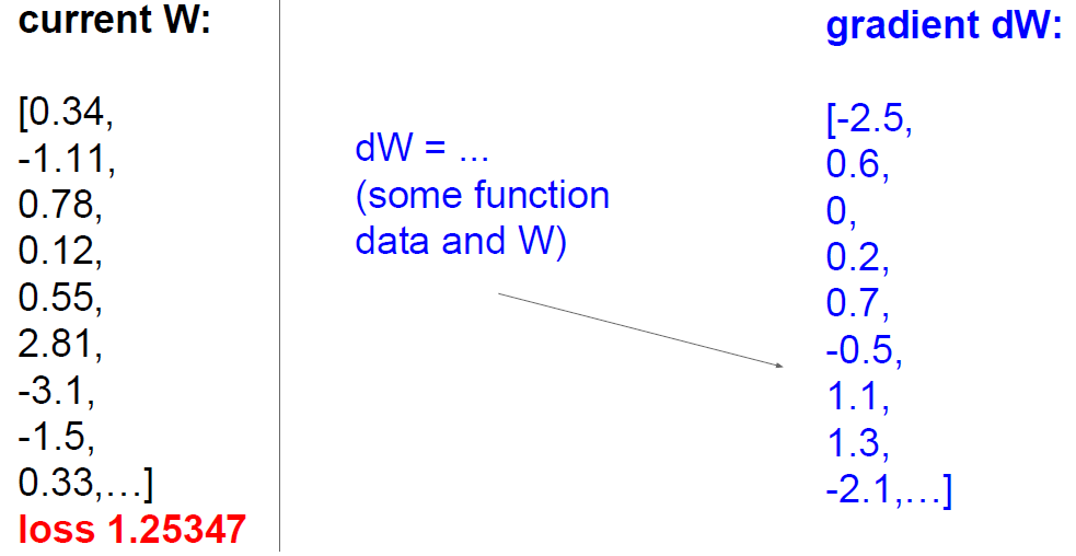
优化的目的是找到合适的W使loss最小，最常用也是最好的办法是Gradient descent。

这里写图片描述
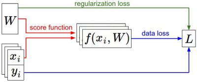
输入参数xi、yi是固定的，W是变化的。
前向传播过程：根据score function计算class score并保存在f()函数中；损失函数包括两部分，（1）根据f和y计算的data loss，（2）regularization loss，是关于W的函数。
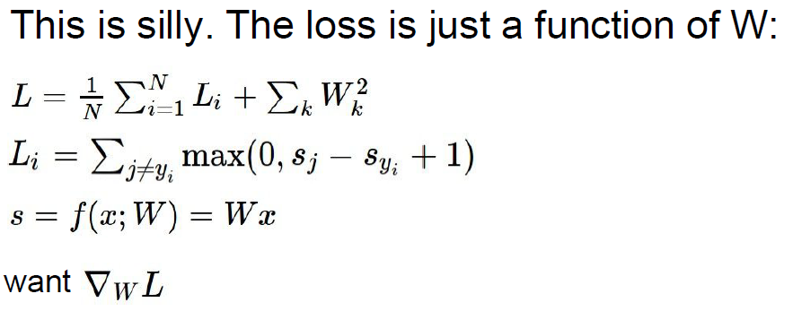
根据变化的W，计算gradient。

下面介绍如何利用梯度计算loss，实现优化W的目的。

解决方法：gradient check。
首先计算Numerically with finite differences，然后计算Analytically with calculus，检验利用Numerically with finite differences计算的loss的准确性。（There are two ways to compute the gradient: A slow, approximate but easy way (numerical gradient), and a fast, exact but more error-prone way that requires calculus (analytic gradient).）

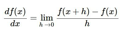
Computing the gradient numerically with finite differences

利用下面公式，并附代码：
这里写图片描述

def eval_numerical_gradient(f, x):
  """ 
  a naive implementation of numerical gradient of f at x 
  - f should be a function that takes a single argument
  - x is the point (numpy array) to evaluate the gradient at
  """ 

  fx = f(x) # evaluate function value at original point
  grad = np.zeros(x.shape)
  h = 0.00001

  # iterate over all indexes in x
  it = np.nditer(x, flags=['multi_index'], op_flags=['readwrite'])
  while not it.finished:

    # evaluate function at x+h
    ix = it.multi_index
    old_value = x[ix]
    x[ix] = old_value + h # increment by h
    fxh = f(x) # evalute f(x + h)
    x[ix] = old_value # restore to previous value (very important!)

    # compute the partial derivative
    grad[ix] = (fxh - fx) / h # the slope
    it.iternext() # step to next dimension

  return grad

通过h的变化得到x，并计算x下的梯度，f(x)对应于L(w+aw)，也就是变化w时候的loss的梯度。

这里写图片描述

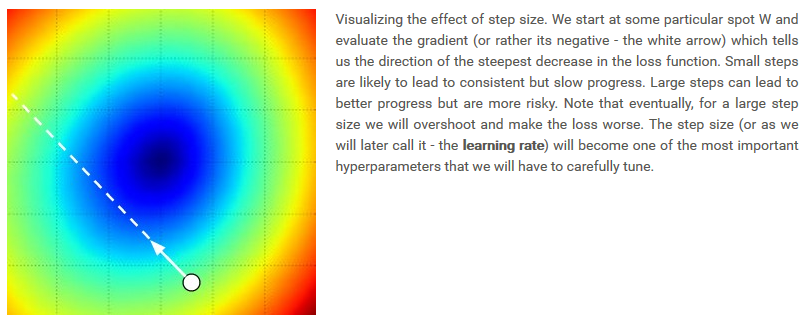
计算loss，受到参数step_size（即learning rate）的限制：给定W，计算loss变化的梯度，这个梯度可以显示loss函数下降的最快的方向，但是不能提供下降到多大程度合适。step_size过大时，收敛速度加快，但是会出现过拟合，是loss变得更坏；当step_size过小时，收敛速度太慢。

这里写图片描述

Computing the gradient analytically with Calculus

通过反向传播计算analytic gradient。

这里写图片描述

Gradient Descent

梯度下降的方法是现在最流行的进行优化的方法，下面是代码。

# Vanilla Gradient Descent

while True:
  weights_grad = evaluate_gradient(loss_fun, data, weights)
  weights += - step_size * weights_grad # perform parameter update

Mini-batch gradient descent.

利用此方法的情况是，样本很大，所以可以去其中的一部分来进行优化。

常用参数设置：
batch_size=32/64/128/…（2的幂）
power=2

# Vanilla Minibatch Gradient Descent

while True:
  data_batch = sample_training_data(data, 256) # sample 256 examples
  weights_grad = evaluate_gradient(loss_fun, data_batch, weights)
  weights += - step_size * weights_grad # perform parameter update

极端情况：当batch_size=1时，这个过程也被称为Stochastic Gradient Descent (SGD) (or also sometimes on-line gradient descent)，但是这种方法不常用，因为计算100个例子的梯度比把1个例子计算100次对于优化更有效。