


【Faster RCNN】损失函数理解:https://blog.csdn.net/Mr_health/article/details/84970776
关于文章中具体一些代码及参数如何得来的请看博客:
tensorflow+faster rcnn代码解析(二):anchor_target_layer、proposal_target_layer、proposal_layer
最近又重新学习了一遍Faster RCNN有挺多收获的,在此重新记录一下。
1. 使用Smoooh L1 Loss的原因
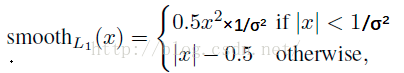
对于边框的预测是一个回归问题。通常可以选择平方损失函数(L2损失)f(x)=x^2。但这个损失对于比较大的误差的惩罚很高。
我们可以采用稍微缓和一点绝对损失函数(L1损失)f(x)=|x|,它是随着误差线性增长,而不是平方增长。但这个函数在0点处导数不存在,因此可能会影响收敛。
一个通常的解决办法是,分段函数,在0点附近使用平方函数使得它更加平滑。它被称之为平滑L1损失函数。它通过一个参数σ 来控制平滑的区域。一般情况下σ = 1,在faster rcnn函数中σ = 3

2. Faster RCNN的损失函数
Faster RCNN的的损失主要分为RPN的损失和Fast RCNN的损失,计算公式如下,并且两部分损失都包括分类损失(cls loss)和回归损失(bbox regression loss)。

下面分别讲一下RPN和fast RCNN部分的损失。
2.1 分类损失
公式:
(1)RPN分类损失:
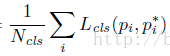
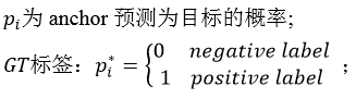
RPN网络的产生的anchor只分为前景和背景,前景的标签为1,背景的标签为0。在训练RPN的过程中,会选择256个anchor,256就是公式中的Ncls
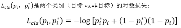
可以看到这是一个这经典的二分类交叉熵损失,对于每一个anchor计算对数损失,然后求和除以总的anchor数量Ncls。这部分的代码tensorflow代码如下:
-
rpn_cls_score = tf.reshape(self._predictions[
'rpn_cls_score_reshape'], [
-1,
2])
#rpn_cls_score = (17100,2)
-
rpn_label = tf.reshape(self._anchor_targets[
'rpn_labels'], [
-1])
#rpn_label = (17100,)
-
rpn_select = tf.where(tf.not_equal(rpn_label,
-1))
#将不等于-1的labels选出来(也就是正负样本选出来),返回序号
-
rpn_cls_score = tf.reshape(tf.gather(rpn_cls_score, rpn_select), [
-1,
2])
#同时选出对应的分数
-
rpn_label = tf.reshape(tf.gather(rpn_label, rpn_select), [
-1])
-
rpn_cross_entropy = tf.reduce_mean(
-
tf.nn.sparse_softmax_cross_entropy_with_logits(logits=rpn_cls_score, labels=rpn_label))
假设我们RPN网络的特征图大小为38×50,那么就会产生38×50×9=17100个anchor,然后在RPN的训练阶段会从17100个anchor中挑选Ncls个anchor用来训练RPN的参数,其中挑选为前景的标签为1,背景的标签为0。
- 代码第一行将其reshape变为(17100,2),行数表示anchor的数量,列数为前景和背景,表示属于前景和背景的分数。
- 代码第二行和第三行,将RPN的label也reshape成(17100,),即分别对应上anchor,然后从中选出不等于-1的,也就是选择出前景和背景,数量为Ncls,返回其index,为rpn_select。
- 代码第四行,根据index选择出对应的分数。
- 第五行,根据rpn_label和rpn_cls_score计算交叉熵损失。其中reduce_mean函数就是除以个数(Ncls)求平均。
(2)Fast RCNN分类损失:
RPN的分类损失时二分类的交叉熵损失,而Fast RCNN是多分类的交叉熵损失(当你训练的类别数>2时,这里假定类别数为5)。在Fast RCNN的训练过程中会选出128个rois,即Ncls = 128,标签的值就是0到4。代码为:
-
cross_entropy =
tf.reduce_mean(
-
tf.nn.sparse_softmax_cross_entropy_with_logits(
-
logits=
tf.reshape(cls_score, [-1, self._num_classes]), labels=label))
2.2 回归损失
回归损失这块就RPN和Fast RCNN一起讲,公式为:

其中:
-
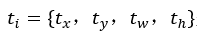 是一个向量,表示anchor,RPN训练阶段(rois,FastRCNN阶段)预测的偏移量。
  是与ti维度相同的向量,表示anchor,RPN训练阶段(rois,FastRCNN阶段)相对于gt实际的偏移量
![]()
R是smoothL1 函数,就是我们上面说的,不同之处是这里σ = 3,RPN训练(σ = 1,Fast RCNN训练),![]()
对于每一个anchor 计算完![]() 部分后还要乘以P*,如前所述,P*有物体时(positive)为1,没有物体(negative)时为0,意味着只有前景才计算损失,背景不计算损失。inside_weights就是这个作用。
部分后还要乘以P*,如前所述,P*有物体时(positive)为1,没有物体(negative)时为0,意味着只有前景才计算损失,背景不计算损失。inside_weights就是这个作用。
对于![]() 和Nreg的解释在RPN训练过程中如下(之所以以RPN训练为前提因为此时batch size = 256,如果是fast rcnn,batchsize = 128):
和Nreg的解释在RPN训练过程中如下(之所以以RPN训练为前提因为此时batch size = 256,如果是fast rcnn,batchsize = 128):
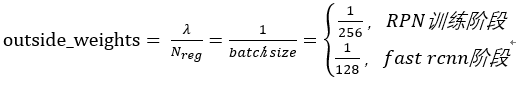
所以 就是outside_weights,没有前景(fg)也没有后景(bg)的为0,其他为1/(bg+fg)=Ncls。
代码:
-
def _smooth_l1_loss(self, bbox_pred, bbox_targets, bbox_inside_weights, bbox_outside_weights, sigma=1.0, dim=[1]):
-
sigma_2 = sigma **
2
-
box_diff = bbox_pred - bbox_targets
#ti-ti*
-
in_box_diff = bbox_inside_weights * box_diff
#前景才有计算损失的资格
-
abs_in_box_diff = tf.abs(in_box_diff)
#x = |ti-ti*|
-
smoothL1_sign = tf.stop_gradient(tf.to_float(tf.less(abs_in_box_diff,
1. / sigma_2)))
#判断smoothL1输入的大小,如果x = |ti-ti*|小于就返回1,否则返回0
-
#计算smoothL1损失
-
in_loss_box = tf.pow(in_box_diff,
2) * (sigma_2 /
2.) * smoothL1_sign + (abs_in_box_diff - (
0.5 / sigma_2)) * (
1. - smoothL1_sign)
-
out_loss_box = bbox_outside_weights * in_loss_box
-
loss_box = tf.reduce_mean(tf.reduce_sum(
-
out_loss_box,
-
axis=dim
-
))
-
return loss_box
一些感悟
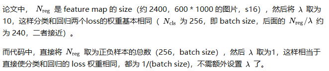
论文中把Ncls,Nreg和![]() 都看做是平衡分类损失和回归损失的归一化权重,但是我在看tensorflow代码实现faster rcnn的损失时发现(这里以fast rcnn部分的分类损失和box回归损失为例,如下),可以看到在计算分类损失时,并没有输入Ncls这个参数,只是在计算box回归损失的时候输入了outside_weights这个参数。这时候我才意识到分类损失是交叉熵函数,求和后会除以总数量,除以Ncls已经包含到交叉熵函数本身。
都看做是平衡分类损失和回归损失的归一化权重,但是我在看tensorflow代码实现faster rcnn的损失时发现(这里以fast rcnn部分的分类损失和box回归损失为例,如下),可以看到在计算分类损失时,并没有输入Ncls这个参数,只是在计算box回归损失的时候输入了outside_weights这个参数。这时候我才意识到分类损失是交叉熵函数,求和后会除以总数量,除以Ncls已经包含到交叉熵函数本身。
为了平衡两种损失的权重,outside_weights的取值取决于Ncls,而Ncls的取值取决于batch_size。因此才会有
-
# RCNN, class loss
-
cls_score =
self._predictions[
"cls_score"]
-
label = tf.reshape(
self._proposal_targets[
"labels"], [-
1])
-
-
cross_entropy = tf.reduce_mean(
-
tf.nn.sparse_softmax_cross_entropy_with_logits(
-
logits=tf.reshape(cls_score, [-
1,
self._num_classes]), labels=label))
-
-
# RCNN, bbox loss
-
bbox_pred =
self._predictions[
'bbox_pred']
#(128,12)
-
bbox_targets =
self._proposal_targets[
'bbox_targets']
#(128,12)
-
bbox_inside_weights =
self._proposal_targets[
'bbox_inside_weights']
#(128,12)
-
bbox_outside_weights =
self._proposal_targets[
'bbox_outside_weights']
#(128,12)
-
-
loss_box =
self._smooth_l1_loss(bbox_pred, bbox_targets, bbox_inside_weights, bbox_outside_weights)
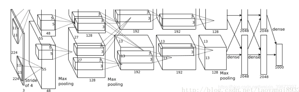
第一个卷积层
输入的图片大小为:224*224*3(或者是227*227*3)
第一个卷积层为:11*11*96即尺寸为11*11,有96个卷积核,步长为4,卷积层后跟ReLU,因此输出的尺寸为 224/4=56,去掉边缘为55,因此其输出的每个feature map 为 55*55*96,同时后面跟LRN层,尺寸不变.
最大池化层,核大小为3*3,步长为2,因此feature map的大小为:27*27*96.
第二层卷积层
输入的tensor为27*27*96
卷积和的大小为: 5*5*256,步长为1,尺寸不会改变,同样紧跟ReLU,和LRN层.
最大池化层,和大小为3*3,步长为2,因此feature map为:13*13*256
第三层至第五层卷积层
输入的tensor为13*13*256
第三层卷积为 3*3*384,步长为1,加上ReLU
第四层卷积为 3*3*384,步长为1,加上ReLU
第五层卷积为 3*3*256,步长为1,加上ReLU
第五层后跟最大池化层,核大小3*3,步长为2,因此feature map:6*6*256
第六层至第八层全连接层
接下来的三层为全连接层,分别为:
1. FC : 4096 + ReLU
2. FC:4096 + ReLU
3. FC: 1000 最后一层为softmax为1000类的概率值.
2. AlexNet中的trick
AlexNet将CNN用到了更深更宽的网络中,其效果分类的精度更高相比于以前的LeNet,其中有一些trick是必须要知道的.
ReLU的应用
AlexNet使用ReLU代替了Sigmoid,其能更快的训练,同时解决sigmoid在训练较深的网络中出现的梯度消失,或者说梯度弥散的问题.
Dropout随机失活
随机忽略一些神经元,以避免过拟合,
重叠的最大池化层
在以前的CNN中普遍使用平均池化层,AlexNet全部使用最大池化层,避免了平均池化层的模糊化的效果,并且步长比池化的核的尺寸小,这样池化层的输出之间有重叠,提升了特征的丰富性.
提出了LRN层
局部响应归一化,对局部神经元创建了竞争的机制,使得其中响应小打的值变得更大,并抑制反馈较小的.
使用了GPU加速计算
使用了gpu加速神经网络的训练
数据增强
使用数据增强的方法缓解过拟合现象.
3. Tensorflow实现AlexNet
-
def print_activations(t):
-
print(t.op.name,
' ', t.get_shape().as_list())
上面的函数为输出当前层的参数的信息.下面是我对开源实现做了一些参数上的修改,代码如下:
-
def inference(images):
-
"""Build the AlexNet model.
-
Args:
-
images: Images Tensor
-
Returns:
-
pool5: the last Tensor in the convolutional component of AlexNet.
-
parameters: a list of Tensors corresponding to the weights and biases of the
-
AlexNet model.
-
"""
-
parameters = []
-
# conv1
-
with tf.name_scope(
'conv1')
as
scope:
-
kernel = tf.Variable(tf.truncated_normal([
11,
11,
3,
96], dtype=tf.float32,
-
stddev=
1e-1),
name=
'weights')
-
conv = tf.nn.conv2d(images, kernel, [
1,
4,
4,
1], padding=
'VALID')
-
biases = tf.Variable(tf.constant(
0.0, shape=[
96], dtype=tf.float32),
-
trainable=
True,
name=
'biases')
-
bias = tf.nn.bias_add(
conv, biases)
-
conv1 = tf.nn.relu(bias,
name=
scope)
-
print_activations(conv1)
-
parameters += [kernel, biases]
-
-
# lrn1
-
# TODO(shlens, jiayq): Add a GPU version of local response normalization.
-
-
# pool1
-
pool1 = tf.nn.max_pool(conv1,
-
ksize=[
1,
3,
3,
1],
-
strides=[
1,
2,
2,
1],
-
padding=
'VALID',
-
name=
'pool1')
-
print_activations(pool1)
-
-
# conv2
-
with tf.name_scope(
'conv2')
as
scope:
-
kernel = tf.Variable(tf.truncated_normal([
5,
5,
96,
256], dtype=tf.float32,
-
stddev=
1e-1),
name=
'weights')
-
conv = tf.nn.conv2d(pool1, kernel, [
1,
1,
1,
1], padding=
'SAME')
-
biases = tf.Variable(tf.constant(
0.0, shape=[
256], dtype=tf.float32),
-
trainable=
True,
name=
'biases')
-
bias = tf.nn.bias_add(
conv, biases)
-
conv2 = tf.nn.relu(bias,
name=
scope)
-
parameters += [kernel, biases]
-
print_activations(conv2)
-
-
# pool2
-
pool2 = tf.nn.max_pool(conv2,
-
ksize=[
1,
3,
3,
1],
-
strides=[
1,
2,
2,
1],
-
padding=
'VALID',
-
name=
'pool2')
-
print_activations(pool2)
-
-
# conv3
-
with tf.name_scope(
'conv3')
as
scope:
-
kernel = tf.Variable(tf.truncated_normal([
3,
3,
256,
384],
-
dtype=tf.float32,
-
stddev=
1e-1),
name=
'weights')
-
conv = tf.nn.conv2d(pool2, kernel, [
1,
1,
1,
1], padding=
'SAME')
-
biases = tf.Variable(tf.constant(
0.0, shape=[
384], dtype=tf.float32),
-
trainable=
True,
name=
'biases')
-
bias = tf.nn.bias_add(
conv, biases)
-
conv3 = tf.nn.relu(bias,
name=
scope)
-
parameters += [kernel, biases]
-
print_activations(conv3)
-
-
# conv4
-
with tf.name_scope(
'conv4')
as
scope:
-
kernel = tf.Variable(tf.truncated_normal([
3,
3,
384,
384],
-
dtype=tf.float32,
-
stddev=
1e-1),
name=
'weights')
-
conv = tf.nn.conv2d(conv3, kernel, [
1,
1,
1,
1], padding=
'SAME')
-
biases = tf.Variable(tf.constant(
0.0, shape=[
384], dtype=tf.float32),
-
trainable=
True,
name=
'biases')
-
bias = tf.nn.bias_add(
conv, biases)
-
conv4 = tf.nn.relu(bias,
name=
scope)
-
parameters += [kernel, biases]
-
print_activations(conv4)
-
-
# conv5
-
with tf.name_scope(
'conv5')
as
scope:
-
kernel = tf.Variable(tf.truncated_normal([
3,
3,
384,
256],
-
dtype=tf.float32,
-
stddev=
1e-1),
name=
'weights')
-
conv = tf.nn.conv2d(conv4, kernel, [
1,
1,
1,
1], padding=
'SAME')
-
biases = tf.Variable(tf.constant(
0.0, shape=[
256], dtype=tf.float32),
-
trainable=
True,
name=
'biases')
-
bias = tf.nn.bias_add(
conv, biases)
-
conv5 = tf.nn.relu(bias,
name=
scope)
-
parameters += [kernel, biases]
-
print_activations(conv5)
-
-
# pool5
-
pool5 = tf.nn.max_pool(conv5,
-
ksize=[
1,
3,
3,
1],
-
strides=[
1,
2,
2,
1],
-
padding=
'VALID',
-
name=
'pool5')
-
print_activations(pool5)
-
-
return pool5,
parameters
-
-
-
def time_tensorflow_run(
session, target, info_string):
-
"""Run the computation to obtain the target tensor and print timing stats.
-
Args:
-
session: the TensorFlow session to run the computation under.
-
target: the target Tensor that is passed to the session's run() function.
-
info_string: a string summarizing this run, to be printed with the stats.
-
Returns:
-
None
-
"""
-
num_steps_burn_in =
10
-
total_duration =
0.0
-
total_duration_squared =
0.0
-
for i
in xrange(FLAGS.num_batches + num_steps_burn_in):
-
start_time = time.time()
-
_ = session.run(target)
-
duration = time.time() - start_time
-
if i >= num_steps_burn_in:
-
if
not i %
10:
-
print (
'%s: step %d, duration = %.3f' %
-
(datetime.now(), i - num_steps_burn_in,
duration))
-
total_duration +=
duration
-
total_duration_squared +=
duration *
duration
-
mn = total_duration / FLAGS.num_batches
-
vr = total_duration_squared / FLAGS.num_batches - mn * mn
-
sd = math.sqrt(vr)
-
print (
'%s: %s across %d steps, %.3f +/- %.3f sec / batch' %
-
(datetime.now(), info_string, FLAGS.num_batches, mn, sd))
-
-
-
测试的函数:
image是随机生成的数据,不是真实的数据
-
def run_benchmark():
-
"""Run the benchmark on AlexNet."""
-
with tf.Graph().as_default():
-
# Generate some dummy images.
-
image_size =
224
-
# Note that our padding definition is slightly different the cuda-convnet.
-
# In order to force the model to start with the same activations sizes,
-
# we add 3 to the image_size and employ VALID padding above.
-
images = tf.Variable(tf.random_normal([FLAGS.batch_size,
-
image_size,
-
image_size,
3],
-
dtype=tf.float32,
-
stddev=
1e-1))
-
-
# Build a Graph that computes the logits predictions from the
-
# inference model.
-
pool5,
parameters = inference(images)
-
-
# Build an initialization operation.
-
init = tf.global_variables_initializer()
-
-
# Start running operations on the Graph.
-
config = tf.ConfigProto()
-
config.gpu_options.allocator_type =
'BFC'
-
sess = tf.Session(config=config)
-
sess.run(init)
-
-
# Run the forward benchmark.
-
time_tensorflow_run(sess, pool5,
"Forward")
-
-
# Add a simple objective so we can calculate the backward pass.
-
objective = tf.nn.l2_loss(pool5)
-
# Compute the gradient with respect to all the parameters.
-
grad = tf.gradients(objective,
parameters)
-
# Run the backward benchmark.
-
time_tensorflow_run(sess, grad,
"Forward-backward")
-
-
-
def
main(_):
-
run_benchmark()
-
-
-
if __name__ ==
'__main__':
-
parser = argparse.ArgumentParser()
-
parser.add_argument(
-
'--batch_size',
-
type=
int,
-
default=
128,
-
help=
'Batch size.'
-
)
-
parser.add_argument(
-
'--num_batches',
-
type=
int,
-
default=
100,
-
help=
'Number of batches to run.'
-
)
-
FLAGS, unparsed = parser.parse_known_args()
-
tf.app.run(
main=
main, argv=[sys.argv[
0]] + unparsed)
输出的结果为:
下面为输出的尺寸,具体的分析过程上面已经说的很详细了.
-
conv1 [
128,
54,
54,
96]
-
pool1 [
128,
26,
26,
96]
-
conv2 [
128,
26,
26,
256]
-
pool2 [
128,
12,
12,
256]
-
conv3 [
128,
12,
12,
384]
-
conv4 [
128,
12,
12,
384]
-
conv5 [
128,
12,
12,
256]
-
pool5 [
128,
5,
5,
256]
下面是训练的前后向耗时,可以看到后向传播比前向要慢3倍.
-
2018-
11-
27
17:
49:
36.
936271: step
0, duration =
0.
085
-
2018-
11-
27
17:
49:
37.
860652: step
10, duration =
0.
085
-
2018-
11-
27
17:
49:
38.
794103: step
20, duration =
0.
100
-
2018-
11-
27
17:
49:
39.
726452: step
30, duration =
0.
099
-
2018-
11-
27
17:
49:
40.
637597: step
40, duration =
0.
088
-
2018-
11-
27
17:
49:
41.
546659: step
50, duration =
0.
078
-
2018-
11-
27
17:
49:
42.
471295: step
60, duration =
0.
085
-
2018-
11-
27
17:
49:
43.
389295: step
70, duration =
0.
095
-
2018-
11-
27
17:
49:
44.
306961: step
80, duration =
0.
085
-
2018-
11-
27
17:
49:
45.
225164: step
90, duration =
0.
085
-
2018-
11-
27
17:
49:
46.
058470: Forward across
100 steps,
0.
092 +/-
0.
008 sec / batch
-
2018-
11-
27
17:
49:
50.
335397: step
0, duration =
0.
281
-
2018-
11-
27
17:
49:
53.
041129: step
10, duration =
0.
279
-
2018-
11-
27
17:
49:
55.
747921: step
20, duration =
0.
269
-
2018-
11-
27
17:
49:
58.
454006: step
30, duration =
0.
269
-
2018-
11-
27
17:
50:
01.
176237: step
40, duration =
0.
285
-
2018-
11-
27
17:
50:
03.
882712: step
50, duration =
0.
269
-
2018-
11-
27
17:
50:
06.
573259: step
60, duration =
0.
269
-
2018-
11-
27
17:
50:
09.
286011: step
70, duration =
0.
270
-
2018-
11-
27
17:
50:
12.
007992: step
80, duration =
0.
275
-
2018-
11-
27
17:
50:
14.
706777: step
90, duration =
0.
262
-
2018-
11-
27
17:
50:
17.
138761: Forward-backward across
100 steps,
0.
271 +/-
0.
006 sec / batch
-
An exception has occurred, use %tb to see the full traceback.


 6409
6409


 被折叠的 条评论
为什么被折叠?
被折叠的 条评论
为什么被折叠?
 到【灌水乐园】发言


