


前言:在Task4,我们学习语义分割的评价函数和各类损失函数,需要掌握常见的评价函数和损失函数Dice、IoU、BCE、Focal Loss、Lovász-Softmax,以及使用不同评价/损失函数进行模型训练。
分类中的TP TN FP FN
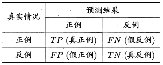
在讲解语义分割中常用的评价函数和损失函数之前,先补充一**TP(真正例 true positive) TN(真反例 true negative) FP(假正例 false positive) FN(假反例 false negative)**的知识。在分类问题中,我们经常看到上述的表述方式,以二分类为例,我们可以将所有的样本预测结果分成TP、TN、 FP、FN四类,并且每一类含有的样本数量之和为总样本数量,即TP+FP+FN+TN=总样本数量。其混淆矩阵如下:
上述的概念都是通过以预测结果的视角定义的,可以依据下面方式理解:
-
预测结果中的正例 → 在实际中是正例 → 的所有样本被称为真正例(TP)<预测正确>
-
预测结果中的正例 → 在实际中是反例 → 的所有样本被称为假正例(FP)<预测错误>
-
预测结果中的反例 → 在实际中是正例 → 的所有样本被称为假反例(FN)<预测错误>
-
预测结果中的反例 → 在实际中是反例 → 的所有样本被称为真反例(TN)<预测正确>
这里就不得不提及精确率(precision)和召回率(recall):
P
r
e
c
i
s
i
o
n
=
T
P
T
P
+
F
P
R
e
c
a
l
l
=
T
P
T
P
+
F
N
Precision=\frac{TP}{TP+FP} \\ Recall=\frac{TP}{TP+FN}
Precision=TP+FPTPRecall=TP+FNTP
P
r
e
c
i
s
i
o
n
Precision
Precision代表了预测的正例中真正的正例所占比例;
R
e
c
a
l
l
Recall
Recall代表了真正的正例中被正确预测出来的比例。
转移到语义分割任务中来,我们可以将语义分割看作是对每一个图像像素的的分类问题。根据混淆矩阵中的定义,我们亦可以将特定像素所属的集合或区域划分成TP、TN、 FP、FN四类。
| target | prediction |
|---|---|
 |  |
| Intersection( T ∩ P T \cap P T∩P) | union( T ∪ P T \cup P T∪P) |
 |  |
以上面的图片为例,图中左子图中的人物区域(黄色像素集合)是我们真实标注的前景信息(target),其他区域(紫色像素集合)为背景信息。当经过预测之后,我们会得到的一张预测结果,图中右子图中的黄色像素为预测的前景(prediction),紫色像素为预测的背景区域。此时,我们便能够将预测结果分成4个部分:
-
预测结果中的黄色无线区域 → 真实的前景 → 的所有像素集合被称为真正例(TP)<预测正确>
-
预测结果中的蓝色斜线区域 → 真实的背景 → 的所有像素集合被称为假正例(FP)<预测错误>
-
预测结果中的红色斜线区域 → 真实的前景 → 的所有像素集合被称为假反例(FN)<预测错误>
-
预测结果中的白色斜线区域 → 真实的背景 → 的所有像素集合被称为真反例(TN)<预测正确>
Dice评价指标
Dice系数
Dice系数(Dice coefficient)是常见的评价分割效果的方法之一,同样也可以改写成损失函数用来度量prediction和target之间的距离。Dice系数定义如下:
D
i
c
e
(
T
,
P
)
=
2
∣
T
∩
P
∣
∣
T
∣
∪
∣
P
∣
=
2
T
P
F
P
+
2
T
P
+
F
N
Dice (T, P) = \frac{2 |T \cap P|}{|T| \cup |P|} = \frac{2TP}{FP+2TP+FN}
Dice(T,P)=∣T∣∪∣P∣2∣T∩P∣=FP+2TP+FN2TP
式中:
T
T
T表示真实前景(target),
P
P
P表示预测前景(prediction)。Dice系数取值范围为
[
0
,
1
]
[0,1]
[0,1],其中值为1时代表预测与真实完全一致。仔细观察,Dice系数与分类评价指标中的F1 score很相似:
1 F 1 = 1 P r e c i s i o n + 1 R e c a l l F 1 = 2 T P F P + 2 T P + F N \frac{1}{F1} = \frac{1}{Precision} + \frac{1}{Recall} \\ F1 = \frac{2TP}{FP+2TP+FN} F11=Precision1+Recall1F1=FP+2TP+FN2TP
所以,Dice系数不仅在直观上体现了target与prediction的相似程度,同时其本质上还隐含了精确率和召回率两个重要指标。
计算Dice时,将
∣
T
∩
P
∣
|T \cap P|
∣T∩P∣近似为prediction与target对应元素相乘再相加的结果。
∣
T
∣
|T|
∣T∣ 和
∣
P
∣
|P|
∣P∣的计算直接进行简单的元素求和(也有一些做法是取平方求和),如下示例:
∣
T
∩
P
∣
=
[
0.01
0.03
0.02
0.02
0.05
0.12
0.09
0.07
0.89
0.85
0.88
0.91
0.99
0.97
0.95
0.97
]
∗
[
0
0
0
0
0
0
0
0
1
1
1
1
1
1
1
1
]
→
[
0
0
0
0
0
0
0
0
0.89
0.85
0.88
0.91
0.99
0.97
0.95
0.97
]
→
s
u
m
7.41
|T \cap P| = \begin{bmatrix} 0.01 & 0.03 & 0.02 & 0.02 \\ 0.05 & 0.12 & 0.09 & 0.07 \\ 0.89 & 0.85 & 0.88 & 0.91 \\ 0.99 & 0.97 & 0.95 & 0.97 \\ \end{bmatrix} * \begin{bmatrix} 0 & 0 & 0 & 0 \\ 0 & 0 & 0 & 0 \\ 1 & 1 & 1 & 1 \\ 1 & 1 & 1 & 1 \\ \end{bmatrix} \stackrel{}{\rightarrow} \begin{bmatrix} 0 & 0 & 0 & 0 \\ 0 & 0 & 0 & 0 \\ 0.89 & 0.85 & 0.88 & 0.91 \\ 0.99 & 0.97 & 0.95 & 0.97 \\ \end{bmatrix} \stackrel{sum}{\rightarrow} 7.41
∣T∩P∣=⎣⎢⎢⎡0.010.050.890.990.030.120.850.970.020.090.880.950.020.070.910.97⎦⎥⎥⎤∗⎣⎢⎢⎡0011001100110011⎦⎥⎥⎤→⎣⎢⎢⎡000.890.99000.850.97000.880.95000.910.97⎦⎥⎥⎤→sum7.41
∣ T ∣ = [ 0.01 0.03 0.02 0.02 0.05 0.12 0.09 0.07 0.89 0.85 0.88 0.91 0.99 0.97 0.95 0.97 ] → s u m 7.82 |T| = \begin{bmatrix} 0.01 & 0.03 & 0.02 & 0.02 \\ 0.05 & 0.12 & 0.09 & 0.07 \\ 0.89 & 0.85 & 0.88 & 0.91 \\ 0.99 & 0.97 & 0.95 & 0.97 \\ \end{bmatrix} \stackrel{sum}{\rightarrow} 7.82 ∣T∣=⎣⎢⎢⎡0.010.050.890.990.030.120.850.970.020.090.880.950.020.070.910.97⎦⎥⎥⎤→sum7.82
∣ P ∣ = [ 0 0 0 0 0 0 0 0 1 1 1 1 1 1 1 1 ] → s u m 8 |P| = \begin{bmatrix} 0 & 0 & 0 & 0 \\ 0 & 0 & 0 & 0 \\ 1 & 1 & 1 & 1 \\ 1 & 1 & 1 & 1 \\ \end{bmatrix} \stackrel{sum}{\rightarrow} 8 ∣P∣=⎣⎢⎢⎡0011001100110011⎦⎥⎥⎤→sum8
Dice Loss
Dice Loss是在V-net模型中被提出应用的,是通过Dice系数转变而来,其实为了能够实现最小化的损失函数,以方便模型训练,以
1
−
D
i
c
e
1 - Dice
1−Dice的形式作为损失函数:
L
=
1
−
2
∣
T
∩
P
∣
∣
T
∣
∪
∣
P
∣
L = 1-\frac{2 |T \cap P|}{|T| \cup |P|}
L=1−∣T∣∪∣P∣2∣T∩P∣
在一些场合还可以添加上Laplace smoothing减少过拟合:
L
=
1
−
2
∣
T
∩
P
∣
+
1
∣
T
∣
∪
∣
P
∣
+
1
L = 1-\frac{2 |T \cap P| + 1}{|T| \cup |P|+1}
L=1−∣T∣∪∣P∣+12∣T∩P∣+1
代码实现
import numpy as np

def dice(output, target):
    '''计算Dice系数'''
    smooth = 1e-6 # 避免0为除数
    intersection = (output * target).sum()
    return (2. * intersection + smooth) / (output.sum() + target.sum() + smooth)

# 生成随机两个矩阵测试
target = np.random.randint(0, 2, (3, 3))
output = np.random.randint(0, 2, (3, 3))

d = dice(output, target)
# ----------------------------
target = array([[1, 0, 0],
       			[0, 1, 1],
			    [0, 0, 1]])
output = array([[1, 0, 1],
       			[0, 1, 0],
       			[0, 0, 0]])
d = 0.5714286326530524
IoU评价指标
IoU(intersection over union)指标就是常说的交并比,不仅在语义分割评价中经常被使用,在目标检测中也是常用的评价指标。顾名思义,交并比就是指target与prediction两者之间交集与并集的比值:
I
o
U
=
T
∩
P
T
∪
P
=
T
P
F
P
+
T
P
+
F
N
IoU=\frac{T \cap P}{T \cup P}=\frac{TP}{FP+TP+FN}
IoU=T∪PT∩P=FP+TP+FNTP
仍然以人物前景分割为例,如下图,其IoU的计算就是使用
i
n
t
e
r
s
e
c
t
i
o
n
/
u
n
i
o
n
intersection / union
intersection/union。
| target | prediction |
|---|---|
| |
| Intersection( T ∩ P T \cap P T∩P) | union( T ∪ P T \cup P T∪P) |
| |
代码实现
def iou_score(output, target):
    '''计算IoU指标'''
	  intersection = np.logical_and(target, output)
    union = np.logical_or(target, output)
    return np.sum(intersection) / np.sum(union)

# 生成随机两个矩阵测试
target = np.random.randint(0, 2, (3, 3))
output = np.random.randint(0, 2, (3, 3))

d = iou_score(output, target)
# ----------------------------
target = array([[1, 0, 0],
       			[0, 1, 1],
			    [0, 0, 1]])
output = array([[1, 0, 1],
       			[0, 1, 0],
       			[0, 0, 0]])
d = 0.4
BCE损失函数
BCE损失函数(Binary Cross-Entropy Loss)是交叉熵损失函数(Cross-Entropy Loss)的一种特例,BCE Loss只应用在二分类任务中。针对分类问题,单样本的交叉熵损失为:
l
(
y
,
y
^
)
=
−
∑
i
=
1
c
y
i
⋅
l
o
g
y
^
i
l(\pmb y, \pmb{\hat y})=- \sum_{i=1}^{c}y_i \cdot log\hat y_i
l(yyy,y^y^y^)=−i=1∑cyi⋅logy^i
式中,
y
=
{
y
1
,
y
2
,
.
.
.
,
y
c
,
}
\pmb{y}=\{y_1,y_2,...,y_c,\}
yyy={y1,y2,...,yc,},其中
y
i
y_i
yi是非0即1的数字,代表了是否属于第
i
i
i类,为真实值;
y
^
i
\hat y_i
y^i代表属于第i类的概率,为预测值。可以看出,交叉熵损失考虑了多类别情况,针对每一种类别都求了损失。针对二分类问题,上述公式可以改写为:
l
(
y
,
y
^
)
=
−
[
y
⋅
l
o
g
y
^
+
(
1
−
y
)
⋅
l
o
g
(
1
−
y
^
)
]
l(y,\hat y)=-[y \cdot log\hat y +(1-y)\cdot log (1-\hat y)]
l(y,y^)=−[y⋅logy^+(1−y)⋅log(1−y^)]
式中,
y
y
y为真实值,非1即0;
y
^
\hat y
y^为所属此类的概率值,为预测值。这个公式也就是BCE损失函数,即二分类任务时的交叉熵损失。值得强调的是,公式中的
y
^
\hat y
y^为概率分布形式,因此在使用BCE损失前,都应该将预测出来的结果转变成概率值,一般为sigmoid激活之后的输出。
代码实现
在pytorch中,官方已经给出了BCE损失函数的API,免去了自己编写函数的痛苦:
torch.nn.BCELoss(weight: Optional[torch.Tensor] = None, size_average=None, reduce=None, reduction: str = 'mean')
ℓ ( y , y ^ ) = L = { l 1 , … , l N } ⊤ , l n = − w n [ y n ⋅ l o g y ^ n + ( 1 − y n ) ⋅ l o g ( 1 − y ^ n ) ] ℓ(y,\hat y)=L=\{l_1,…,l_N \}^⊤,\ \ \ l_n=-w_n[y_n \cdot log\hat y_n +(1-y_n)\cdot log (1-\hat y_n)] ℓ(y,y^)=L={l1,…,lN}⊤, ln=−wn[yn⋅logy^n+(1−yn)⋅log(1−y^n)]
参数:
weight(Tensor)- 为每一批量下的loss添加一个权重,很少使用
size_average(bool)- 弃用中
reduce(bool)- 弃用中
reduction(str) - ‘none’ | ‘mean’ | ‘sum’:为代替上面的size_average和reduce而生。——为mean时返回的该批量样本loss的平均值;为sum时,返回的该批量样本loss之和
同时,pytorch还提供了已经结合了Sigmoid函数的BCE损失:torch.nn.BCEWithLogitsLoss(),相当于免去了实现进行Sigmoid激活的操作。
import torch
import torch.nn as nn

bce = nn.BCELoss()
bce_sig = nn.BCEWithLogitsLoss()

input = torch.randn(5, 1, requires_grad=True)
target = torch.empty(5, 1).random_(2)
pre = nn.Sigmoid()(input)

loss_bce = bce(pre, target)
loss_bce_sig = bce_sig(input, target)

# ------------------------
input = tensor([[-0.2296],
        		[-0.6389],
        		[-0.2405],
        		[ 1.3451],
        		[ 0.7580]], requires_grad=True)
output = tensor([[1.],
        		 [0.],
        		 [0.],
        		 [1.],
        		 [1.]])
pre = tensor([[0.4428],
        	  [0.3455],
        	  [0.4402],
        	  [0.7933],
        	  [0.6809]], grad_fn=<SigmoidBackward>)

print(loss_bce)
tensor(0.4869, grad_fn=<BinaryCrossEntropyBackward>)

print(loss_bce_sig)
tensor(0.4869, grad_fn=<BinaryCrossEntropyWithLogitsBackward>)
Focal Loss
Focal loss最初是出现在目标检测领域,主要是为了解决正负样本比例失调的问题。那么对于分割任务来说,如果存在数据不均衡的情况,也可以借用focal loss来进行缓解。Focal loss函数公式如下所示:
l
o
s
s
=
−
1
N
∑
i
=
1
N
(
α
y
i
(
1
−
p
i
)
γ
log
p
i
+
(
1
−
α
)
(
1
−
y
i
)
p
i
γ
log
(
1
−
p
i
)
)
loss = -\frac{1}{N} \sum_{i=1}^{N}\left(\alpha y_{i}\left(1-p_{i}\right)^{\gamma} \log p_{i}+(1-\alpha)\left(1-y_{i}\right) p_{i}^{\gamma} \log \left(1-p_{i}\right)\right)
loss=−N1i=1∑N(αyi(1−pi)γlogpi+(1−α)(1−yi)piγlog(1−pi))
仔细观察就不难发现,它其实是BCE扩展而来,对比BCE其实就多了个
α
(
1
−
p
i
)
γ
和
(
1
−
α
)
p
i
γ
\alpha(1-p_{i})^{\gamma}和(1-\alpha)p_{i}^{\gamma}
α(1−pi)γ和(1−α)piγ
为什么多了这个就能缓解正负样本不均衡的问题呢?见下图:
[外链图片转存失败,源站可能有防盗链机制,建议将图片保存下来直接上传(img-FBZVFTAQ-1614614871349)(img/Task4:评价函数与损失函数_image/FocalLoss.png)]
简单来说: α α α解决样本不平衡问题, γ γ γ解决样本难易问题。
也就是说,当数据不均衡时,可以根据比例设置合适的 α α α,这个很好理解,为了能够使得正负样本得到的损失能够均衡,因此对loss前面加上一定的权重,其中负样本数量多,因此占用的权重可以设置的小一点;正样本数量少,就对正样本产生的损失的权重设的高一点。
那γ具体怎么起作用呢?以图中 γ = 5 γ=5 γ=5曲线为例,假设 g t gt gt类别为1,当模型预测结果为1的概率 p t p_t pt比较大时,我们认为模型预测的比较准确,也就是说这个样本比较简单。而对于比较简单的样本,我们希望提供的loss小一些而让模型主要学习难一些的样本,也就是 p t → 1 p_t→ 1 pt→1则loss接近于0,既不用再特别学习;当分类错误时, p t → 0 p_t → 0 pt→0则loss正常产生,继续学习。对比图中蓝色和绿色曲线,可以看到,γ值越大,当模型预测结果比较准确的时候能提供更小的loss,符合我们为简单样本降低loss的预期。
代码实现:
import torch.nn as nn
import torch
import torch.nn.functional as F

class FocalLoss(nn.Module):
    def __init__(self, alpha=1, gamma=2, logits=False, reduce=True):
        super(FocalLoss, self).__init__()
        self.alpha = alpha
        self.gamma = gamma
        self.logits = logits	# 如果BEC带logits则损失函数在计算BECloss之前会自动计算softmax/sigmoid将其映射到[0,1]
        self.reduce = reduce

    def forward(self, inputs, targets):
        if self.logits:
            BCE_loss = F.binary_cross_entropy_with_logits(inputs, targets, reduce=False)
        else:
            BCE_loss = F.binary_cross_entropy(inputs, targets, reduce=False)
        pt = torch.exp(-BCE_loss)
        F_loss = self.alpha * (1-pt)**self.gamma * BCE_loss

        if self.reduce:
            return torch.mean(F_loss)
        else:
            return F_loss

# ------------------------

FL1 = FocalLoss(logits=False)
FL2 = FocalLoss(logits=True)

inputs = torch.randn(5, 1, requires_grad=True)
targets = torch.empty(5, 1).random_(2)
pre = nn.Sigmoid()(inputs)

f_loss_1 = FL1(pre, targets)
f_loss_2 = FL2(inputs, targets)

# ------------------------

print('inputs:', inputs)
inputs: tensor([[-1.3521],
        [ 0.4975],
        [-1.0178],
        [-0.3859],
        [-0.2923]], requires_grad=True)

print('targets:', targets)
targets: tensor([[1.],
        [1.],
        [0.],
        [1.],
        [1.]])

print('pre:', pre)
pre: tensor([[0.2055],
        [0.6219],
        [0.2655],
        [0.4047],
        [0.4274]], grad_fn=<SigmoidBackward>)

print('f_loss_1:', f_loss_1)
f_loss_1: tensor(0.3375, grad_fn=<MeanBackward0>)

print('f_loss_2', f_loss_2)
f_loss_2 tensor(0.3375, grad_fn=<MeanBackward0>)
Lovász-Softmax
IoU是评价分割模型分割结果质量的重要指标,因此很自然想到能否用 1 − I o U 1-IoU 1−IoU(即Jaccard loss)来做损失函数,但是它是一个离散的loss,不能直接求导,所以无法直接用来作为损失函数。为了克服这个离散的问题,可以采用lLovász extension将离散的Jaccard loss 变得连续,从而可以直接求导,使得其作为分割网络的loss function。Lovász-Softmax相比于交叉熵函数具有更好的效果。
论文地址:
首先明确定义,在语义分割任务中,给定真实像素标签向量
y
∗
\pmb{y^*}
y∗y∗y∗和预测像素标签
y
^
\pmb{\hat{y}}
y^y^y^,则所属类别
c
c
c的IoU(也称为Jaccard index)如下,其取值范围为
[
0
,
1
]
[0,1]
[0,1],并规定
0
/
0
=
1
0/0=1
0/0=1:
J
c
(
y
∗
,
y
^
)
=
∣
{
y
∗
=
c
}
∩
{
y
^
=
c
}
∣
∣
{
y
∗
=
c
}
∪
{
y
^
=
c
}
∣
J_c(\pmb{y^*},\pmb{\hat{y}})=\frac{|\{\pmb{y^*}=c\} \cap \{\pmb{\hat{y}}=c\}|}{|\{\pmb{y^*}=c\} \cup \{\pmb{\hat{y}}=c\}|}
Jc(y∗y∗y∗,y^y^y^)=∣{y∗y∗y∗=c}∪{y^y^y^=c}∣∣{y∗y∗y∗=c}∩{y^y^y^=c}∣
则Jaccard loss为:
Δ
J
c
(
y
∗
,
y
^
)
=
1
−
J
c
(
y
∗
,
y
^
)
\Delta_{J_c}(\pmb{y^*},\pmb{\hat{y}}) =1-J_c(\pmb{y^*},\pmb{\hat{y}})
ΔJc(y∗y∗y∗,y^y^y^)=1−Jc(y∗y∗y∗,y^y^y^)
针对类别
c
c
c,所有未被正确预测的像素集合定义为:
M
c
(
y
∗
,
y
^
)
=
{
y
∗
=
c
,
y
^
≠
c
}
∪
{
{
y
∗
≠
c
,
y
^
=
c
}
}
M_c(\pmb{y^*},\pmb{\hat{y}})=\{\pmb{y^*}=c, \pmb{\hat{y}} \neq c\}\cup \{\{\pmb{y^*}\neq c, \pmb{\hat{y}} = c\}\}
Mc(y∗y∗y∗,y^y^y^)={y∗y∗y∗=c,y^y^y^=c}∪{{y∗y∗y∗=c,y^y^y^=c}}
则可将Jaccard loss改写为关于
M
c
M_c
Mc的子模集合函数(submodular set functions):
Δ
J
c
:
M
c
∈
{
0
,
1
}
p
↦
∣
M
c
∣
∣
{
y
∗
=
c
}
∪
M
c
∣
\Delta_{J_c}:M_c \in \{0,1\}^{p} \mapsto \frac{|M_c|}{|\{\pmb{y^*}=c\}\cup M_c|}
ΔJc:Mc∈{0,1}p↦∣{y∗y∗y∗=c}∪Mc∣∣Mc∣
方便理解,此处可以把
{
0
,
1
}
p
\{0,1\}^p
{0,1}p理解成如图像mask展开成离散一维向量的形式。
Lovász extension可以求解子模最小化问题,并且子模的Lovász extension是凸函数,可以高效实现最小化。在论文中作者对 Δ \Delta Δ(集合函数)和 Δ ‾ \overline{\Delta} Δ(集合函数的Lovász extension)进行了定义,为不涉及过多概念以方便理解,此处不再过多讨论。我们可以将 Δ ‾ \overline{\Delta} Δ理解为一个线性插值函数,可以将 { 0 , 1 } p \{0,1\}^p {0,1}p这种离散向量连续化,主要是为了方便后续反向传播、求梯度等等。因此我们可以通过这个线性插值函数得到 Δ J c \Delta_{J_c} ΔJc的Lovász extension Δ J c ‾ \overline{\Delta_{J_c}} ΔJc。
在具有
c
(
c
>
2
)
c(c>2)
c(c>2)个类别的语义分割任务中,我们使用Softmax函数将模型的输出映射到概率分布形式,类似传统交叉熵损失函数所进行的操作:
p
i
(
c
)
=
e
F
i
(
c
)
∑
c
′
∈
C
e
F
i
(
c
′
)
∀
i
∈
[
1
,
p
]
,
∀
c
∈
C
p_i(c)=\frac{e^{F_i(c)}}{\sum_{c^{'}\in C}e^{F_i(c^{'})}} \forall i \in [1,p],\forall c \in C
pi(c)=∑c′∈CeFi(c′)eFi(c) ∀i∈[1,p],∀c∈C
式中,
p
i
(
c
)
p_i(c)
pi(c)表示了像素
i
i
i所属类别
c
c
c的概率。通过上式可以构建每个像素产生的误差
m
(
c
)
m(c)
m(c):
m
i
(
c
)
=
{
1
−
p
i
(
c
)
,
i
f
c
=
y
i
∗
p
i
(
c
)
,
o
t
h
e
r
w
i
s
e
m_i(c)=\left \{ \begin{array}{c} 1-p_i(c),\ \ if \ \ c=y^{*}_{i} \\ p_i(c),\ \ \ \ \ \ \ otherwise \end{array} \right.
mi(c)={1−pi(c), if c=yi∗pi(c), otherwise
可知,对于一张图像中所有像素则误差向量为
m
(
c
)
∈
{
0
,
1
}
p
m(c)\in \{0, 1\}^p
m(c)∈{0,1}p,则可以建立关于
Δ
J
c
\Delta_{J_c}
ΔJc的代理损失函数:
l
o
s
s
(
p
(
c
)
)
=
Δ
J
c
‾
(
m
(
c
)
)
loss(p(c))=\overline{\Delta_{J_c}}(m(c))
loss(p(c))=ΔJc(m(c))
当我们考虑整个数据集是,一般会使用mIoU进行度量,因此我们对上述损失也进行平均化处理,则定义的Lovász-Softmax损失函数为:
l
o
s
s
(
p
)
=
1
∣
C
∣
∑
c
∈
C
Δ
J
c
‾
(
m
(
c
)
)
loss(\pmb{p})=\frac{1}{|C|}\sum_{c\in C}\overline{\Delta_{J_c}}(m(c))
loss(ppp)=∣C∣1c∈C∑ΔJc(m(c))
代码实现
论文作者已经给出了Lovász-Softmax实现代码,并且有pytorch和tensorflow两种版本,并提供了使用demo。此处将针对多分类任务的Lovász-Softmax源码进行展示。
Lovász-Softmax实现链接:https://github.com/bermanmaxim/LovaszSoftmax
import torch
from torch.autograd import Variable
import torch.nn.functional as F
import numpy as np
try:
    from itertools import  ifilterfalse
except ImportError: # py3k
    from itertools import  filterfalse as ifilterfalse

# --------------------------- MULTICLASS LOSSES ---------------------------
def lovasz_softmax(probas, labels, classes='present', per_image=False, ignore=None):
    """
    Multi-class Lovasz-Softmax loss
      probas: [B, C, H, W] Variable, class probabilities at each prediction (between 0 and 1).
              Interpreted as binary (sigmoid) output with outputs of size [B, H, W].
      labels: [B, H, W] Tensor, ground truth labels (between 0 and C - 1)
      classes: 'all' for all, 'present' for classes present in labels, or a list of classes to average.
      per_image: compute the loss per image instead of per batch
      ignore: void class labels
    """
    if per_image:
        loss = mean(lovasz_softmax_flat(*flatten_probas(prob.unsqueeze(0), lab.unsqueeze(0), ignore), classes=classes)
                          for prob, lab in zip(probas, labels))
    else:
        loss = lovasz_softmax_flat(*flatten_probas(probas, labels, ignore), classes=classes)
    return loss


def lovasz_softmax_flat(probas, labels, classes='present'):
    """
    Multi-class Lovasz-Softmax loss
      probas: [P, C] Variable, class probabilities at each prediction (between 0 and 1)
      labels: [P] Tensor, ground truth labels (between 0 and C - 1)
      classes: 'all' for all, 'present' for classes present in labels, or a list of classes to average.
    """
    if probas.numel() == 0:
        # only void pixels, the gradients should be 0
        return probas * 0.
    C = probas.size(1)
    losses = []
    class_to_sum = list(range(C)) if classes in ['all', 'present'] else classes
    for c in class_to_sum:
        fg = (labels == c).float() # foreground for class c
        if (classes is 'present' and fg.sum() == 0):
            continue
        if C == 1:
            if len(classes) > 1:
                raise ValueError('Sigmoid output possible only with 1 class')
            class_pred = probas[:, 0]
        else:
            class_pred = probas[:, c]
        errors = (Variable(fg) - class_pred).abs()
        errors_sorted, perm = torch.sort(errors, 0, descending=True)
        perm = perm.data
        fg_sorted = fg[perm]
        losses.append(torch.dot(errors_sorted, Variable(lovasz_grad(fg_sorted))))
    return mean(losses)


def flatten_probas(probas, labels, ignore=None):
    """
    Flattens predictions in the batch
    """
    if probas.dim() == 3:
        # assumes output of a sigmoid layer
        B, H, W = probas.size()
        probas = probas.view(B, 1, H, W)
    B, C, H, W = probas.size()
    probas = probas.permute(0, 2, 3, 1).contiguous().view(-1, C)  # B * H * W, C = P, C
    labels = labels.view(-1)
    if ignore is None:
        return probas, labels
    valid = (labels != ignore)
    vprobas = probas[valid.nonzero().squeeze()]
    vlabels = labels[valid]
    return vprobas, vlabels


def xloss(logits, labels, ignore=None):
    """
    Cross entropy loss
    """
    return F.cross_entropy(logits, Variable(labels), ignore_index=255)

# --------------------------- HELPER FUNCTIONS ---------------------------
def isnan(x):
    return x != x

def mean(l, ignore_nan=False, empty=0):
    """
    nanmean compatible with generators.
    """
    l = iter(l)
    if ignore_nan:
        l = ifilterfalse(isnan, l)
    try:
        n = 1
        acc = next(l)
    except StopIteration:
        if empty == 'raise':
            raise ValueError('Empty mean')
        return empty
    for n, v in enumerate(l, 2):
        acc += v
    if n == 1:
        return acc
    return acc / n
课后作业
- 理解各类评价函数的原理;
- 对比各类损失函数原理,并进行具体实践;


 3501
3501


 被折叠的 条评论
为什么被折叠?
被折叠的 条评论
为什么被折叠?
 到【灌水乐园】发言


