


1. 本文目的
使用SVM代替CNN网络的全连接层,即CNN提取特征后利用SVM进行分类。(注:仍使用完整CNN网络进行训练获取卷积层参数,SVM参数单独训练获得,后续会对此进行详细说明。)
2. 实验流程:
- 对样本数据进行处理
- 建立完整的卷积神经网络(CNN)
- 利用训练数据进行训练,获取卷积层权重参数
- 将卷积层输出转换为SVM输入特征向量
- 利用上一步特征向量对SVM进行训练
- 利用测试数据进行准确率测试。
3. 网络结构
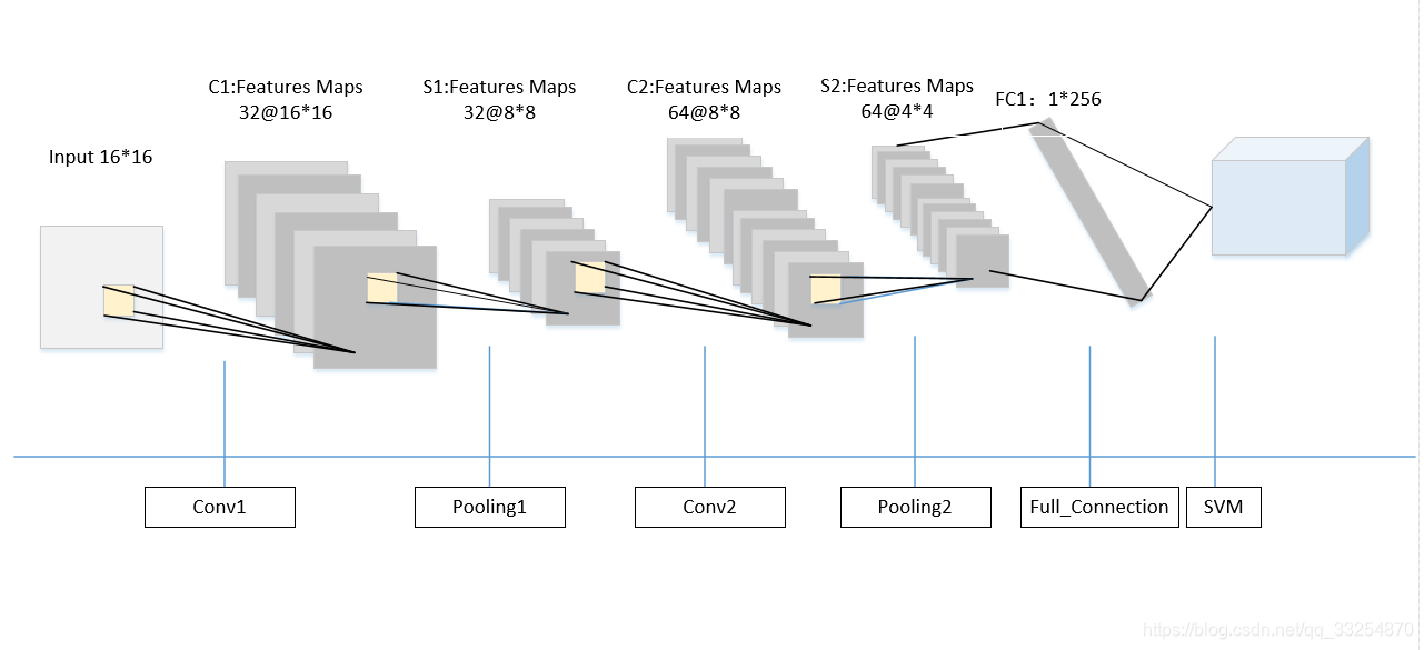
CNN有两个卷积层,两个全连接层,其中卷积层卷积核大小为5 * 5,步长为1,池化层卷积核大小为2 * 2,第一个全连接层输出h_fc1转化为特征向量输入SVM。
feature map大小变化如表所示:
| Conv1 | Pooling1 | Conv2 | Pooling2 | Full_Connectin1 | SVM | |
|---|---|---|---|---|---|---|
| input size | 16*16 | 16*16 | 8*8 | 8*8 | 4 * 4 * 64 | 1* 256 |
| filter | 5*5 | 2*2 | 5*5 | 2*2 | - | - |
| output size | 16 * 16 | 8*8 | 8*8 | 4*4 | 256 | - |
4. 核心代码
# coding=utf8
import random
import numpy as np
import tensorflow as tf
from sklearn import svm

for file_num in range(10):
    # 在十个随机生成的不相干数据集上进行测试,将结果综合
    print('testing NO.%d dataset.......' % file_num)
    f1 = open('digit_train_' + file_num.__str__() + '.data')
    lines1 = f1.readlines()
    # 训练数据
    X_train = []
    y_train = []
    y_train_temp = []
    y_train_transform = []
    for i in range(len(lines1)):
        X_train.append(list(map(int, map(float, lines1[i].split(' ')[:256]))))
        y_train.append(list(map(int, lines1[i].split(' ')[256:266])))
        y_train_transform.append(np.argmax(list(map(int, lines1[i].split(' ')[256:266]))))
    f1.close()

    f2 = open('digit_test_' + file_num.__str__() + '.data')
    lines2 = f2.readlines()
    # 测试数据
    X_test = []
    y_test = []
    y_test_transform = []
    for i in range(len(lines2)):
        X_test.append(list(map(int, map(float, lines2[i].split(' ')[:256]))))
        y_test.append(list(map(int, lines2[i].split(' ')[256:266])))
        y_test_transform.append(np.argmax(list(map(int, lines2[i].split(' ')[256:266]))))
    f2.close()

    # 建立一个tensorflow的会话
    sess = tf.InteractiveSession()

    # 初始化权值向量
    def weight_variable(shape):
        initial = tf.truncated_normal(shape, stddev=0.1)
        return tf.Variable(initial)

    # 初始化偏置向量
    def bias_variable(shape):
        initial = tf.constant(0.1, shape=shape)
        return tf.Variable(initial)

    # 二维卷积运算,步长为1,输出大小不变
    def conv2d(x, W):
        return tf.nn.conv2d(x, W, strides=[1, 1, 1, 1], padding='SAME')

    # 池化运算,将卷积特征缩小为1/2
    def max_pool_2x2(x):
        return tf.nn.max_pool(x, ksize=[1, 2, 2, 1], strides=[1, 2, 2, 1], padding='SAME')


    # 给x,y留出占位符,以便未来填充数据
    x = tf.placeholder("float", [None, 256])
    y_ = tf.placeholder("float", [None, 10])

    # 第一个卷积层,5x5的卷积核,输出向量是32维
    w_conv1 = weight_variable([5, 5, 1, 32])
    b_conv1 = bias_variable([32])
    x_image = tf.reshape(x, [-1, 16, 16, 1])
    # 图片大小是16*16,,-1代表其他维数自适应
    h_conv1 = tf.nn.relu(conv2d(x_image, w_conv1) + b_conv1)
    h_pool1 = max_pool_2x2(h_conv1)
    # 采用的最大池化,因为都是1和0,平均池化没有什么意义

    # 第二层卷积层,输入向量是32维,输出64维,还是5x5的卷积核
    w_conv2 = weight_variable([5, 5, 32, 64])
    b_conv2 = bias_variable([64])

    h_conv2 = tf.nn.relu(conv2d(h_pool1, w_conv2) + b_conv2)
    h_pool2 = max_pool_2x2(h_conv2)

    # 全连接层的w和b
    w_fc1 = weight_variable([4 * 4 * 64, 256])
    b_fc1 = bias_variable([256])
    # 此时输出的维数是256维
    h_pool2_flat = tf.reshape(h_pool2, [-1, 4 * 4 * 64])
    h_fc1 = tf.nn.relu(tf.matmul(h_pool2_flat, w_fc1) + b_fc1)
    # h_fc1是提取出的256维特征,很关键。后面就是用这个输入到SVM中

    # 设置dropout,否则很容易过拟合
    keep_prob = tf.placeholder("float")
    h_fc1_drop = tf.nn.dropout(h_fc1, keep_prob)

    # 输出层,在本实验中只利用它的输出反向训练CNN,至于其具体数值我不关心
    w_fc2 = weight_variable([256, 10])
    b_fc2 = bias_variable([10])

    y_conv = tf.nn.softmax(tf.matmul(h_fc1_drop, w_fc2) + b_fc2)
    cross_entropy = -tf.reduce_sum(y_ * tf.log(y_conv))
    # 设置误差代价以交叉熵的形式
    train_step = tf.train.AdamOptimizer(1e-4).minimize(cross_entropy)
    # 用adma的优化算法优化目标函数
    correct_prediction = tf.equal(tf.argmax(y_conv, 1), tf.argmax(y_, 1))
    accuracy = tf.reduce_mean(tf.cast(correct_prediction, "float"))
    sess.run(tf.global_variables_initializer())
    for i in range(1000):
        # 进行1000轮迭代,每次随机从训练样本中抽出50个进行训练
        batch = ([], [])
        p = np.random.choice(range(795), 50, replace=False)
        for k in p:
            batch[0].append(X_train[k])
            batch[1].append(y_train[k])
        if i % 100 == 0:
            train_accuracy = accuracy.eval(feed_dict={x: batch[0], y_: batch[1], keep_prob: 1.0})
            # print "step %d, train accuracy %g" % (i, train_accuracy)
        train_step.run(feed_dict={x: batch[0], y_: batch[1], keep_prob: 0.6})
        # 设置dropout的参数为0.6,测试得到,大点收敛的慢,小点立刻出现过拟合

    print("test accuracy %g" % accuracy.eval(feed_dict={x: X_test, y_: y_test, keep_prob: 1.0}))

    # 将原来的x带入训练好的CNN中计算出来全连接层的特征向量,将结果作为SVM中的特征向量
    x_temp1 = []
    for g in X_train:
        x_temp1.append(sess.run(h_fc1, feed_dict={x: np.array(g).reshape((1, 256))})[0])
        # x_temp1 = preprocessing.scale(x_temp)  # normalization
    x_temp2 = []
    for g in X_test:
        x_temp2.append(sess.run(h_fc1, feed_dict={x: np.array(g).reshape((1, 256))})[0])

    clf = svm.SVC(C=0.9, kernel='linear')  # linear kernel
    clf.fit(x_temp1, y_train_transform)
    # SVM选择了RBF核,C选择了0.9
    print('svm testing accuracy:')
    print(clf.score(x_temp2, y_test_transform))

    sess.close()
注:使用留出法,进行了10次训练与测试过程。
项目源码:https://github.com/dhuQChen/MathematicalModeling/tree/master/CNN_SVM


 2万+
2万+

 被折叠的 条评论
为什么被折叠?
被折叠的 条评论
为什么被折叠?
 到【灌水乐园】发言


