机器学习 day2 线性回归

导三方库：

import pandas as pd 
import numpy as np 
import matplotlib.pyplot as plt

import seaborn as sns

from sklearn.datasets import fetch_california_housing

导入数据集

house = fetch_california_housing()

X = pd.DataFrame(house.data,columns= house.feature_names)
X.head()

	MedInc	HouseAge	AveRooms	AveBedrms	Population	AveOccup	Latitude	Longitude
0	8.3252	41.0	6.984127	1.023810	322.0	2.555556	37.88	-122.23
1	8.3014	21.0	6.238137	0.971880	2401.0	2.109842	37.86	-122.22
2	7.2574	52.0	8.288136	1.073446	496.0	2.802260	37.85	-122.24
3	5.6431	52.0	5.817352	1.073059	558.0	2.547945	37.85	-122.25
4	3.8462	52.0	6.281853	1.081081	565.0	2.181467	37.85	-122.25

数据说明：

MedInc：该街区住户的收入中位数
HouseAge：该街区房屋使用年代的中位数
AveRooms：该街区平均的房间数目
AveBedrms：该街区平均的卧室数目
Population： 街区人口
AveOccup： 平均入住率
Latitude： 街区的纬度
Longitude：街区的经度

房子价值的中位数

house.target # array([4.526, 3.585, 3.521, ..., 0.923, 0.847, 0.894])

数据预处理

检查数据相关性

sns.heatmap(X.corr()
           ,annot=True
            ,center=0
            ,linewidths=0.8
           )

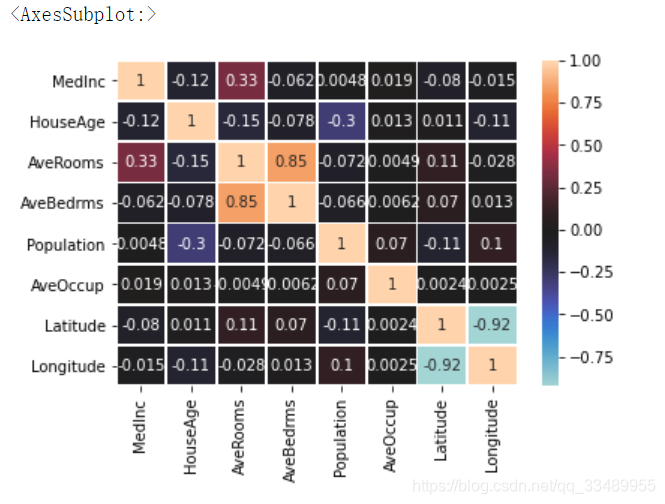
由于经纬度的相关性较高，为保证各变量线性无关，只保留其中一个变量

删除 Latitude

X.drop(columns='Latitude',inplace=True)

数据的标准化

划分数据集：

from sklearn.model_selection import train_test_split
xtrain,xtest,ytrain,ytest = train_test_split(X,house.target)

数据标准化

$$\frac{x_i-\bar{x}}{std}$$

0-1 缩放

$$\frac{x_i-x_{min}}{x_{max}-x_{min}}$$

标准化数据：

from sklearn.preprocessing import StandardScaler

std保存了每一个特征的平均值和标准差

std = StandardScaler().fit(xtrain)

xtrain_

xtrain_ = pd.DataFrame(std.transform(xtrain),columns= X.columns)
xtrain_

xtest_ 此处有疑问

xtest_ = pd.DataFrame(std.transform(xtest),columns= X.columns)
xtest_

数据的0-1缩放

步骤：实例化，fit（）传参，transform转化

from sklearn.preprocessing import MinMaxScaler

mm = MinMaxScaler().fit(xtrain)

xtrain_mm = mm.transform(xtrain)
xtest_mm = mm.transform(xtest)

线性回归（标准化之后的）

导入包

from sklearn.linear_model import Lasso
from sklearn.linear_model import Ridge
from sklearn.linear_model import LinearRegression

初始化：

Lasso_ = Lasso(alpha=1.0, max_iter=5000,tol=0.0001)
#L1 正则  max_iter : 梯度下降最多的迭代次数， tol ：收敛域

Ridge_ = Ridge(alpha=1.0,tol=0.0001)
#L2 正则

LR = LinearRegression(fit_intercept=True)
# 常规线性回归

Lasso回归：

Lasso_.fit(xtrain_,ytrain)# 标准化的xtrain

# Lasso(max_iter=5000)

Lasso_.coef_ # array([ 0.,  0.,  0., -0., -0., -0., -0.])

Ridge 回归：

Ridge_.fit(xtrain_,ytrain) # Ridge(tol=0.0001)

Ridge_.coef_ 

# array([ 1.01918834,  0.20957514, -0.4967906 ,  0.44822796,  0.02923409, -0.06038656, -0.03551321]) 

常规线性回归：

LR.fit(xtrain_,ytrain) # LinearRegression()

LR.coef_

# array([ 1.01948766,  0.20957077, -0.4973972 ,  0.44878819,  0.02922805, -0.06039858, -0.03553571])

线性回归（0-1缩放之后的）

模型评估（标准化之后的）

from sklearn.metrics import mean_squared_error

计算回归误差

LASSO 回归的误差：

mean_squared_error(ytest,Lasso_.predict(xtest_))

结果：1.3495937394960946

Ridge 回归的误差：

mean_squared_error(ytest,Ridge_.predict(xtest_))

结果：0.6598541912416058

常规线性回归误差：

mean_squared_error(ytest,LR.predict(xtest_))

结果：0.6598326497351307

决定系数：R^2

Lasso_.score(xtest_,ytest)

结果：-0.00012336012803904062

Ridge_.score(xtest_,ytest)

结果：0.5110116684554803

LR.score(xtest_,ytest)

结果：0.5110276318992988

模型评估（0-1缩放之后的）

作业：处理波士顿房价数据集