优化问题-LP，QP和QCQP（线性规划，Linear Programming； 二次规划，Quadratic Programming；二次约束二次规划）

线性规划（LP）

LP问题的一般形式为：
$$\begin{array}{ll}\min & {\mathbf{c}}^T\mathbf{x}\\ \text{ s.t. }& \mathbf{G}\mathbf{x}⪯\mathbf{h}\end{array}（6.1）$$
本质：LP问题即是在多面体上找到一个可行解使得线性目标函数最小。

LP的一般形式可以转化为标准形式，即引入松弛变量：
$$\mathbf{s}\triangleq \mathbf{h}-\mathbf{G}\mathbf{x}$$
作为助变量。则（6.1）可以表示为：
$$\begin{array}{ll}\min & {\mathbf{c}}^T\mathbf{x}\\ \text{ s.t. }& \mathbf{s}⪰0,\mathbf{h}-\mathbf{G}\mathbf{x}=\mathbf{s}\end{array}（6.2）$$
进一步：$\mathrm{x}={\mathrm{x}}_{+}-{\mathrm{x}}_{-}$，其中${\mathrm{x}}_{+},{\mathrm{x}}_{-}⪰0$，则（6.2）可以等价为：
$$\begin{array}{ll}\min & \left[\begin{array}{lll}{\mathbf{c}}^T& -{\mathbf{c}}^T& 0^T\end{array}\right]\left[\begin{array}{c}{\mathbf{x}}_{+}\\ {\mathbf{x}}_{-}\\ \mathbf{s}\end{array}\right]\\ \text{ s.t. }& \left[\begin{array}{c}{\mathrm{x}}_{+}\\ {\mathrm{x}}_{-}\\ \mathrm{s}\end{array}\right]⪰0,\left[\begin{array}{lll}\mathbf{G}& -\mathbf{G}& \mathbf{I}\end{array}\right]\left[\begin{array}{c}{\mathrm{x}}_{+}\\ {\mathrm{x}}_{-}\\ \mathrm{s}\end{array}\right]=\mathrm{h}\end{array}（6.3）$$
（6.3）可以重新表示为标准LP形式：
$$\begin{array}{ll}\min & {\mathbf{c}}^T\mathbf{x}\\ \text{ s.t. }& \mathbf{x}⪰0,\mathbf{A}\mathbf{x}=\mathbf{b}\end{array}$$
其中
$$\mathbf{A}=\left[\begin{array}{lll}\mathbf{G}& -\mathbf{G}& \mathbf{I}\end{array}\right],c={\left[{\mathbf{c}}^T-{\mathbf{c}}^T{0}^T\right]}^T,x={\left[{\mathbf{x}}_{+}^T{\mathbf{x}}_{-}^T{\mathbf{s}}^T\right]}^T$$
其中$\mathbf{x}$是未知变量。

LP的一些例子：

Chebyshev中心

考虑欧式球 B ( x c , r ) = { x ∣ ∥ x − x c ∥ 2 ≤ r } B\left(\mathbf{x}_{c}, r\right)=\left\{\mathbf{x} \mid\left\|\mathbf{x}-\mathbf{x}_{c}\right\|_{2} \leq r\right\} B(xc​,r)={ x∣∥x−xc​∥2​≤r}以及多面体 P = { x ∣ a i T x ≤ b i , i = 1 , … , m } \mathcal{P}=\{\mathbf{x} \mid\left.\mathbf{a}_{i}^{T} \mathbf{x} \leq b_{i}, i=1, \ldots, m\right\} P={ x∣aiT​x≤bi​,i=1,…,m}

Chebyshev问题描述为，在多面体$\mathcal{P}$中找到最大的欧式球，如下图所示。该问题表示为：

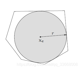
$$\begin{array}{rl}{\max }_{{\mathbf{x}}_c,r}& r\\ \text{ s.t. }& B\left({\mathbf{x}}_c,r\right)\subseteq \mathcal{P}=\left\{\mathbf{x}\mid {\mathbf{a}}_i^T\mathbf{x}\le b_i,i=1,\dots ,m\right\}\end{array}（6.6）$$
该问题看起来是非凸的，但可以转化为LP。考虑欧式球的另一种定义：
B ( x c , r ) = { x c + u ∣ ∥ u ∥ 2 ≤ r } B\left(\mathbf{x}_{c}, r\right)=\left\{\mathbf{x}_{c}+\mathbf{u} \mid\|\mathbf{u}\|_{2} \leq r\right\} B(xc​,r)={ xc​+u∣∥u∥2​≤r}

考虑Cauchy-Schwartz inequality：有：
$${\mathbf{a}}_i^T\mathbf{u}\le {\Vert {\mathbf{a}}_i\Vert }_2\cdot \Vert \mathbf{u}{\Vert }_2$$
考虑（6.6）的约束集可以重新表示为：
$$\begin{array}{rl}B\left({\mathrm{x}}_c,r\right)\subseteq \mathcal{P}& ⟺\sup \left\{{\mathbf{a}}_i^T\left({\mathrm{x}}_c+\mathbf{u}\right)\mid \Vert \mathbf{u}{\Vert }_2\le r\right\}\le b_i,\forall i\\ & ⟺{\mathbf{a}}_i^T{\mathbf{x}}_c+r{\Vert {\mathbf{a}}_i\Vert }_2\le b_i,\forall i\text{ (i.e., }\mathbf{u}=r\Vert {\mathbf{a}}_i\end{array}$$