服装图片分类（tensorflow实现）

from __future__ import absolute_import, division, print_function, unicode_literals
import tensorflow as tf
from tensorflow import keras
import numpy as np
import matplotlib.pyplot as plt
print(tf.__version__)

2.0.0

导入Fashion MNIST 数据集

数据集包含70000灰度图片，10个分类
每张图片的像素为28*28
60000张图片作为训练集，10000张图片作为测试机

fashion_mnist = keras.datasets.fashion_mnist
(train_images, train_labels), (test_images, test_labels) = fashion_mnist.load_data()

class_names = ['T-shirt/top', 'Trouser', 'Pullover', 'Dress', 'Coat',
               'Sandal', 'Shirt', 'Sneaker', 'Bag', 'Ankle boot']

train_images.shape

(60000, 28, 28)

len(train_labels)

60000

train_labels

array([9, 0, 0, ..., 3, 0, 5], dtype=uint8)

test_images.shape

(10000, 28, 28)

len(test_labels)

10000

plt.figure()
plt.imshow(train_images[0])
plt.colorbar()  # 颜色渐变条
plt.grid(False)  # 不添加网格线
plt.show()

数据预处理。图片的像素值范围在0-255，为了使输入数据值在0-1之间，将原始值除以255.0

train_images = train_images / 255.0
test_images = test_images / 255.0

plt.figure(figsize=(10,10))
for i in range(25):
    plt.subplot(5,5,i+1)  # 将图片划分为5行5列
    # 控制每个图片的边框刻度
    plt.xticks([])
    plt.yticks([])
    plt.imshow(train_images[i], cmap=plt.cm.binary)  # 黑白图片
    plt.xlabel(class_names[train_labels[i]])
plt.show()

# 建立网络架构
model = keras.Sequential([
    keras.layers.Flatten(input_shape=(28, 28)),  # 输入数据向量化
    keras.layers.Dense(128, activation='relu'),  # 添加全连接层  
    keras.layers.Dense(10, activation='softmax')
])

# 定义正则化、损失函数
model.compile(optimizer='adam',
             loss='sparse_categorical_crossentropy',
             metrics=['accuracy'])

model.fit(train_images, train_labels, epochs=10)  # 训练网络

Train on 60000 samples
Epoch 1/10
60000/60000 [==============================] - 9s 149us/sample - loss: 0.4946 - accuracy: 0.8247
Epoch 2/10
60000/60000 [==============================] - 7s 116us/sample - loss: 0.3722 - accuracy: 0.8654
Epoch 3/10
60000/60000 [==============================] - 7s 114us/sample - loss: 0.3353 - accuracy: 0.8776
Epoch 4/10
60000/60000 [==============================] - 7s 115us/sample - loss: 0.3116 - accuracy: 0.8846
Epoch 5/10
60000/60000 [==============================] - 8s 126us/sample - loss: 0.2951 - accuracy: 0.8914
Epoch 6/10
60000/60000 [==============================] - 7s 111us/sample - loss: 0.2809 - accuracy: 0.8975
Epoch 7/10
60000/60000 [==============================] - 7s 110us/sample - loss: 0.2716 - accuracy: 0.8988
Epoch 8/10
60000/60000 [==============================] - 7s 118us/sample - loss: 0.2560 - accuracy: 0.9050
Epoch 9/10
60000/60000 [==============================] - 7s 122us/sample - loss: 0.2456 - accuracy: 0.9077
Epoch 10/10
60000/60000 [==============================] - 9s 143us/sample - loss: 0.2385 - accuracy: 0.9110

<tensorflow.python.keras.callbacks.History at 0x29df5dfa780>

test_loss, test_acc = model.evaluate(test_images, test_labels, verbose=2)
print('\nTest accuracy:', test_acc)

10000/1 - 1s - loss: 0.3204 - accuracy: 0.8783
Test accuracy: 0.8783

predictions = model.predict(test_images)
predictions[0]

array([1.2773737e-08, 1.6460965e-09, 1.2608050e-08, 2.2927955e-10,
       8.7082235e-09, 1.5253473e-04, 7.7240850e-07, 5.0626141e-03,
       1.9821150e-07, 9.9478382e-01], dtype=float32)

np.argmax(predictions[0])

9

test_labels[0]

9

def plot_image(i, predictions_array, true_label, img):
    predictions_array, true_label, img = predictions_array, true_label[i], img[i]
    plt.grid(False)
    plt.xticks([])
    plt.yticks([])
    
    plt.imshow(img, cmap=plt.cm.binary)
    
    predicted_label = np.argmax(predictions_array)
    # 预测正确标记为蓝色，错误则为红色
    if predicted_label == true_label:
        color = 'blue'
    else:
        color = 'red'
    # 横轴上分别为 预测的分类名，预测分类的可能性，正确分类名 
    plt.xlabel("{} {:2.0f}% ({})".format(class_names[predicted_label],
                                         100*np.max(predictions_array),
                                         class_names[true_label]),
                                           color=color)

def plot_value_array(i, predictions_array, train_labels):
    predictions_array, true_label = predictions_array, train_labels[i]
    plt.grid(False)
    plt.xticks(range(10))
    plt.yticks([])
    # 直方图横坐标0-9，纵坐标对应每个分类的得分
    thisplot = plt.bar(range(10), predictions_array, color="#777777")
    plt.ylim([0, 1])
    predicted_label = np.argmax(predictions_array)  # 预测的分类标签
    
    thisplot[predicted_label].set_color('red')  # 预测分类的纵坐标标注为红色
    thisplot[true_label].set_color('blue') # 正确分类的纵坐标标注为蓝色

# 第一张图片的预测结果
i = 0
plt.figure(figsize=(6,3))
plt.subplot(1,2,1)
plot_image(i, predictions[i], test_labels, test_images)
plt.subplot(1,2,2)
plot_value_array(i, predictions[i], test_labels)
plt.show()

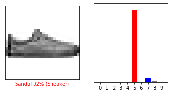
# 第13张图片的预测结果
i = 12
plt.figure(figsize=(6,3))
plt.subplot(1,2,1)
plot_image(i, predictions[i], test_labels, test_images)
plt.subplot(1,2,2)
plot_value_array(i, predictions[i], test_labels)
plt.show()

num_rows = 5
num_cols = 3
num_images = num_rows*num_cols
plt.figure(figsize=(2*2*num_cols, 2*num_rows))
for i in range(num_images):
    plt.subplot(num_rows, 2*num_cols, 2*i+1)  # 每个数据预测结果的第一张图片
    plot_image(i, predictions[i], test_labels, test_images)
    plt.subplot(num_rows, 2*num_cols, 2*i+2)  # 每个数据预测结果的第一张图片
    plot_value_array(i, predictions[i], test_labels)
plt.tight_layout()  # 会自动调整子图参数，使之填充整个图像区域
plt.show()

img = test_images[1]
print(img.shape)

(28, 28)

# 图片添加进空的数据集，这个数据集只有一个数据
img = (np.expand_dims(img,0))  
print(img.shape)

(1, 28, 28)

predictions_single = model.predict(img)
print(predictions_single)

[[8.1730264e-05 7.7724135e-16 9.9977332e-01 2.8166874e-10 1.3929847e-04
  1.6422478e-14 5.6340227e-06 3.3765748e-19 8.4485353e-12 6.8645493e-16]]

plot_value_array(1, predictions_single[0], test_labels)
_ = plt.xticks(range(10), class_names, rotation=45)

np.argmax(predictions_single[0])

2