Prophet代码实战（二）季节项调节

Prophet Quick Start

数据格式

Prophet 的输入必须包含两列的数据框：ds 和 y 。

• ds 列必须包含日期（YYYY-MM-DD）或者是具体的时间点（YYYY-MM-DD HH:MM:SS）。
• y 列必须是数值变量，表示我们希望去预测的量。

example_wp_log_peyton_manning.csv下载地址：

import pandas as pd
from prophet import Prophet

# 读入数据集
df = pd.read_csv('data/example_wp_log_peyton_manning.csv')

print(df.tail(5))
"""
              ds          y
2900  2016-01-16   7.817223
2901  2016-01-17   9.273878
2902  2016-01-18  10.333775
2903  2016-01-19   9.125871
2904  2016-01-20   8.891374
"""

建模流程

通过使用辅助的方法 Prophet.make_future_dataframe 来将未来的日期扩展指定的天数，得到一个合规的数据框。

m = Prophet()
m.fit(df)
# 构建待预测日期数据框，periods = 365 代表除历史数据的日期外再往后推 365 天
horizon = 365
future = m.make_future_dataframe(periods=horizon)
future.tail(5)
"""
             ds
3265 2017-01-15
3266 2017-01-16
3267 2017-01-17
3268 2017-01-18
3269 2017-01-19
"""
# 预测
forecast = m.predict(future)
# 通过 Prophet.plot 方法传入预测得到的数据框，可以对预测的效果进行绘图。
fig1 = m.plot(forecast)
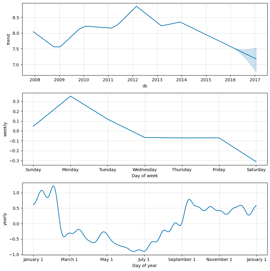
# 使用 Prophet.plot_components 方法。默认情况下，将展示趋势、时间序列的年度季节性和周季节性。如果之前包含了节假日，也会展示出来。
fig2 = m.plot_components(forecast)

如果想查看预测的成分分析，可以使用 Prophet.plot_components 方法。默认情况下，将展示趋势、时间序列的年度季节性和周季节性。如果之前包含了节假日，也会展示出来。

Prophet详解

在上一篇文章【Prophet代码实战（一）趋势项调节】介绍了Prophet算法的趋势项。接下来我们开始介绍Prophet算法的季节项

季节性

Prophet的内置季节性

• yearly_seasonality,是否需要拟合数据中的yearly季节性，以及yearly季节性的傅里叶级数项数。当训练集中有超过1年的数据时，默认为10，
  一般来说拟合yearly的季节性建议至少有一年的数据。

• yearly_seasonality越大，拟合的季节性曲线波动幅度越大

• yearly_seasonality=0或者为False时，表示不拟合yearly季节性。

• 类似还有weekly_seasonaliyt和daily_seasonality。

# 调整yearly_seasonality
m = Prophet(yearly_seasonality=20) 
m.fit(df)
horizon = 365
future = m.make_future_dataframe(periods=horizon)
forecast = m.predict(future)
fig = m.plot_components(forecast)

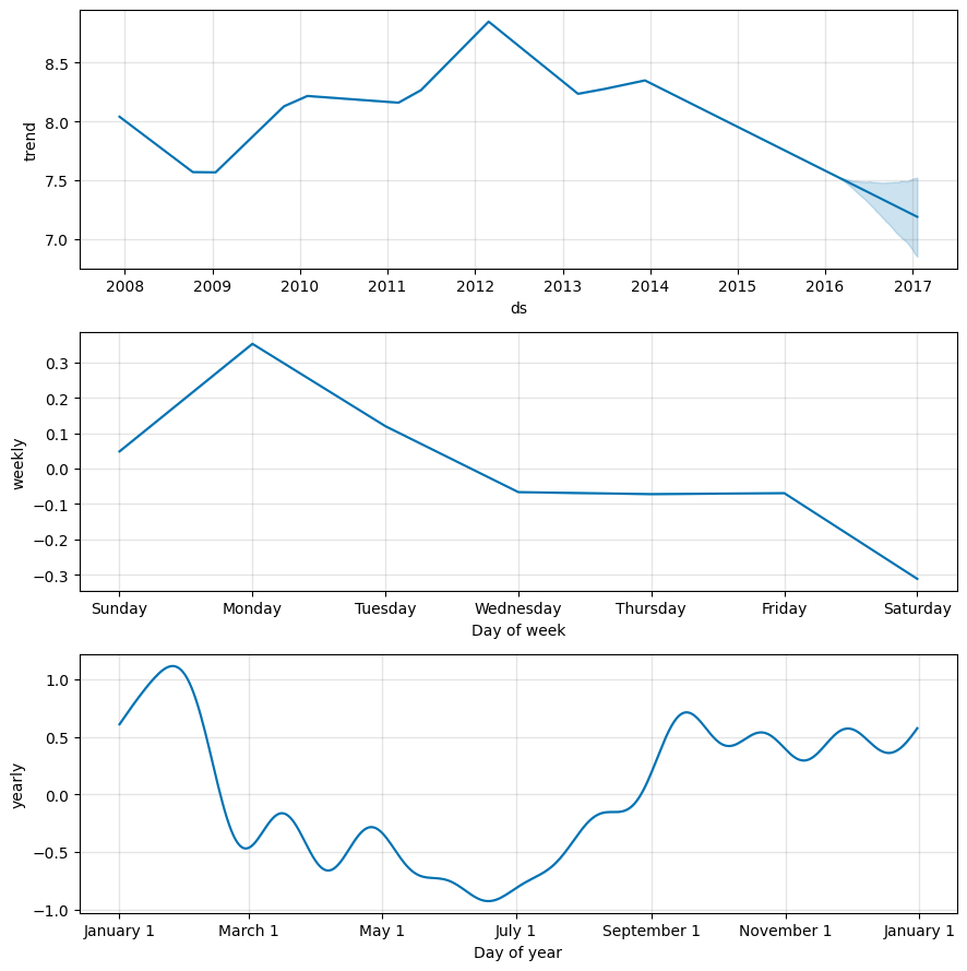
关闭yearly_seasonality

m = Prophet(yearly_seasonality=0) 
m.fit(df)
horizon = 365
future = m.make_future_dataframe(periods=horizon)
forecast = m.predict(future)
fig = m.plot_components(forecast)

超参数seasonality_prior_scale

• 小数，季节性曲线的系数先验概率，默认值为10
• 理论上，seasonality_prior_scale越大，季节性曲线波动越大，越容易过拟合

# 调整seasonality_prior_scale = 10
m = Prophet(seasonality_prior_scale = 10) 
m.fit(df)
horizon = 365
future = m.make_future_dataframe(periods=horizon)
forecast = m.predict(future)
fig = m.plot_components(forecast)

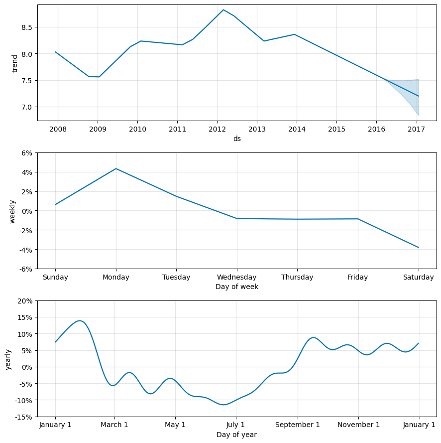
季节性的加法模式和乘法模式
超参数seasonality_mode

• “additive”:默认值，表示季节性对观测值是加法的作用，即y = trend + seasonality
• “multiplicative”:表示季节性对观测值是乘法作用，即y = trend * seasonality
• 一般business相关的时间序列只要选取"multiplicative"
• multiplicative和additive可以通过对数操作相互转化。即 y = trend * seasonality
  可以表示为log(y) = log(trend) + log(seasonality)

# 调整seasonality_mode
m = Prophet(seasonality_mode="multiplicative") 
m.fit(df)
horizon = 365
future = m.make_future_dataframe(periods=horizon)
forecast = m.predict(future)
fig = m.plot_components(forecast)

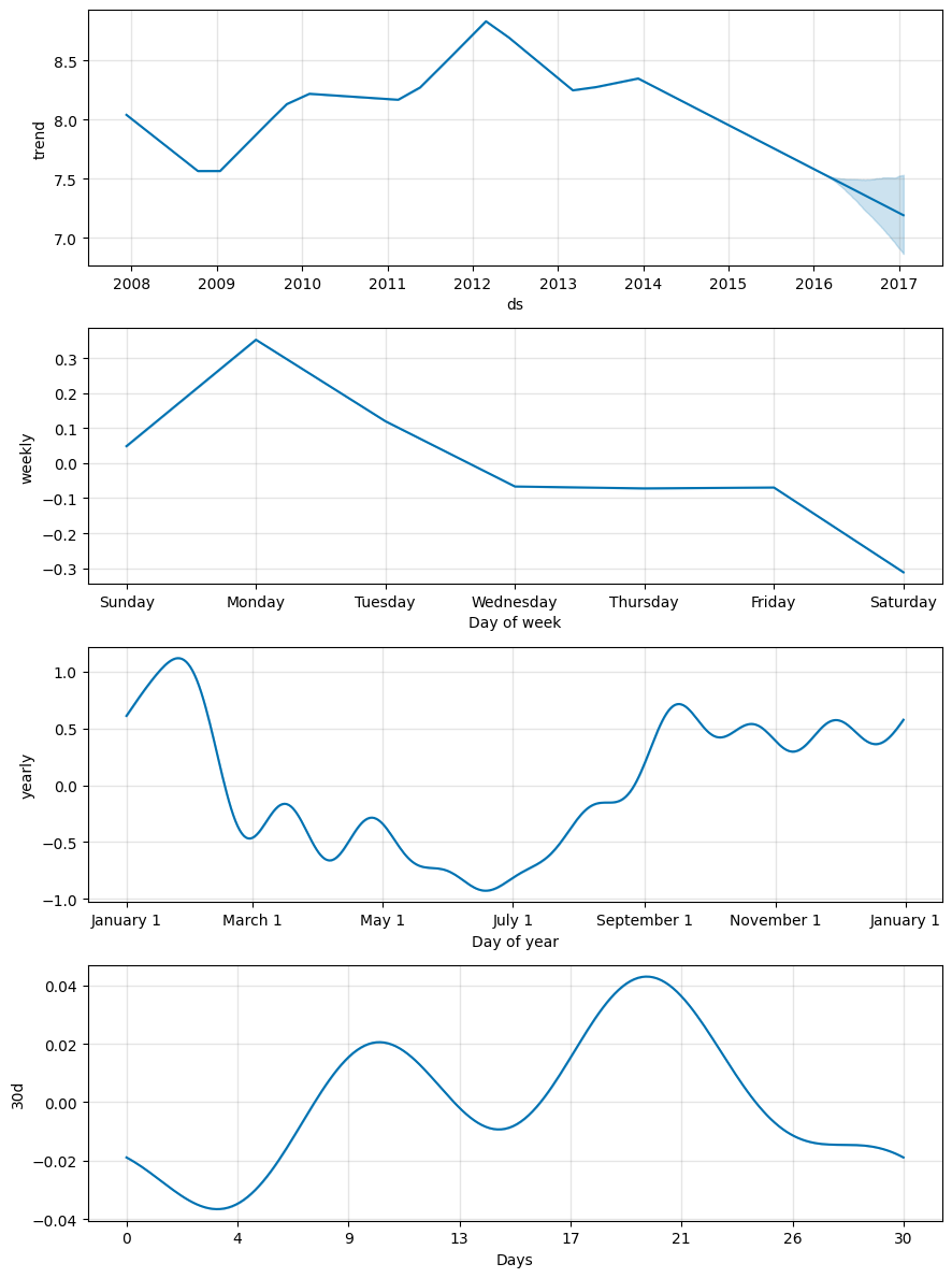
自定义季节性
通过函数add_seasonality()增加新的季节性，参数有：

• name:名称
• period：周期长度
• fourier_order：傅里叶级数项数
• prior_scale：傅里叶系数先验概率

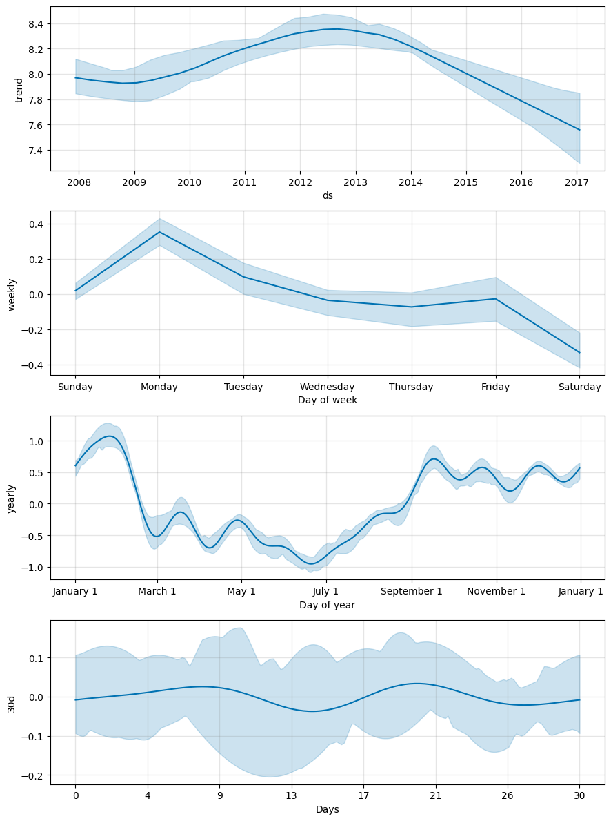
# 通过函数add_seasonality()增加新的季节性
m = Prophet() 
m.add_seasonality(name='30d',period=30,fourier_order=3,prior_scale=0.1)
m.fit(df)
horizon = 365
future = m.make_future_dataframe(periods=horizon)
forecast = m.predict(future)
fig = m.plot_components(forecast)

季节性的置信区间
超参数mcmc_samples,计算置信区间时的蒙特卡洛样本数量

• 默认情况下，Prophet只会返回趋势的置信区间，为了得到季节性的置信区间，我们需要做完全的贝叶斯抽样，采用是通过蒙特卡洛方法完成的。
• mcmc_samples越大，样本越具有代表性，置信区间越准，运算时间也会越久

# 通过mcmc_samples参数返回季节性趋势
m = Prophet(mcmc_samples=30) 
m.add_seasonality(name='30d',period=30,fourier_order=3,prior_scale=0.1)
m.fit(df)
horizon = 365
future = m.make_future_dataframe(periods=horizon)
forecast = m.predict(future)
fig = m.plot_components(forecast)