


本文是做为一个纯新手小白,对下文做的笔记:
R语言聚类分析–cluster, factoextra
后续发现有一个很靠谱的英文教程,收到了相关R包的官方推荐:
datanovia教程
里面分了如下几个课,详细讲了相关理论和API。
因此本文变成了这两个教程的笔记。二者大体相似,略有区别。
目录
标准化
scale(X, center = TRUE, scale = TRUE)对数据集进行标准化。
(标准化就是减去均值再除以标准差,标准化后均值为0,方差为1.)
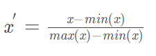
注意还有一个东西是min-max归一化,
我这里scale的参数X用的是一个table类型。
center是是否中心化(减均值),scale是center的基础上是否标准化(除以标准差)
PCA画图
参考此文
fviz_pca_ind(prcomp(df), title = “PCA - my data”,
geom = “point”, ggtheme = theme_classic())
感觉是分隔四类左右:
中间,左,右上,右下,

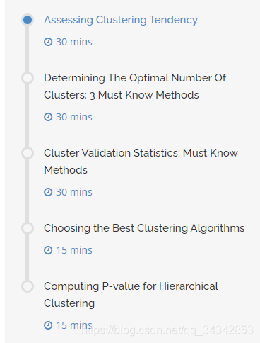
聚类趋势评估(Assessing Clustering Tendency)
Hopkins Statistic 介绍
需要注意的是,网上有两种不同的说法。
说法一
说法二
说法一很奇怪,不太对的亚子。
找到两个比较权威的,都支持说法二,包括该函数的R包的官方文档:
靠谱教程
R包官方文档
估计聚类趋势(assessing clustering tendency)是指对于给定的数据集,评估该数据集是否存在非随机结构。因为:盲目地在数据集上使用聚类方法将返回一些簇,所挖掘的簇可能是误导。数据集上的聚类分析是有意义的,仅当数据中存在非随机结构。
霍普金斯统计量(Hopkins Statistic)是一种空间统计量,检验空间分布的变量的空间随机性。(Han, Kamber, and Pei 2012)
计算步骤:
首先,从所有样本中随机找n个点,然后为每一个点在样本空间中找到一个离他最近的点,并计算它们之间的距离xi,从而得到距离向量x1,x2,…,xn;
然后,从样本的可能取值范围内随机生成n个点,对每一个随机生产的点,找到一个离它最近的样本点,并计算它们之间的距离,得到y1,y2,…,yn。
霍普金斯统计量H可以表示为:

如果样本接近随机分布,那么 ∑ x i \sum x_i ∑xi 和 ∑ y i \sum y_i ∑yi 的取值会比较接近,即H的值接近于0.5;如果聚类趋势明显,则随机生成的样本点y距离应该远大于实际样本点的距离x,即 H的值接近于1. (这里选这个:A value for H higher than 0.75 indicates a clustering tendency at the 90% confidence level.)(这一点在R包factoextra的关让文档里得到证实)
R语言实现
有两种方法,一个是factoextra包的:get_clust_tendency()方法,结果是一个有两个元素(hopkins_stat & plot)的list。用 hierarchical clustering画图。
另一种是hopkins() function [in clustertend package].不画图
方法一:factoextra包的:get_clust_tendency()方法
res = get_clust_tendency(df, 40, graph = TRUE)
res$hopkins_stat # 这行代码会给出下面这个图

图的解释
这个图是啥意思呢,
首先看那个datanovia的靠谱教程:
visual assessment of cluster tendency (VAT) approach 算法(Bezdek and Hathaway, 2002) is as follow:
- Compute the dissimilarity (DM) matrix between the objects in the data set using the Euclidean distance measure
- Reorder the DM so that similar objects are close to one another. This process create an ordered dissimilarity matrix (ODM)
- The ODM is displayed as an ordered dissimilarity image (ODI), which is the visual output of VAT
For the visual assessment of clustering tendency, we start by computing the dissimilarity matrix between observations using the function dist(). Next the function fviz_dist() [factoextra package] is used to display the dissimilarity matrix.
- Red: high similarity (ie: low dissimilarity) | Blue: low similarity。
就是说,VAT方法(聚类趋势可视化评估)实际上是把ODI(排序后的相异性图像)画出来。

如有疑问,再看factoextra包官方文档:
- An ordered dissimilarity image (ODI) is shown. Objects belonging to the same cluster are displayed in consecutive order using hierarchical clustering.
- The VAT detects the clustering tendency in a visual form by counting the number of square shaped dark (or colored) blocks along the diagonal in a VAT image.
- plot for ordered dissimilarity image. This is generated using the function fviz_dist(dist.obj)
只有这三句话相关,意思也是一样的。红色相似。
结合我们的图的结果,可以看到总体上是有一个大的亚型,其他的再说。(其实有点像异常数据和常见数据,而非亚型)
方法二: clustertend包的hopkins()方法
另一种是hopkins() function [in clustertend package].不画图,直接算。通常就用第一种方法就行。
聚类个数选择
理论
回到datanovia教程。
关于聚类个数选择
- 聚类个数的选择,方法很多,不下30多种。
- 没有一个最好的完美方法,所有方法都相对主观。
- 下面介绍常用的几种方法。

这部分中文资料也可以直接参考上文的说法一,也就是此文
肘方法(elbow method):
给定k>0,使用像K-means这样的算法对数据集聚类,并计算簇内方差和var(k) (也叫the total within-cluster sum of square (wss))。然后,绘制var关于k的曲线。曲线的第一个(或最显著的)拐点暗示“正确的”簇数。
交叉验证法:将数据分为m部分;用m-1部分获得聚类模型,余下部分评估聚类质量(测试样本与类中心的距离和);对k>0重复m次,比较总体质量,选择能获得最好聚类质量的k
测定聚类质量:在数据集上使用聚类方法之后,需要评估结果簇的质量。
Average silhouette method
同肘方法,只不过把计算wws换成计算Average silhouette,把拐点换成最大值。(average silhouette的取最大的时候是最好的)
Gap statistic method
先按k1,k2,…, kn 聚类,然后求出within intra-cluster variation Wk.
在新建一个随机均匀分布的数据集,按k1,k2,…, kn 聚类,然后求出within intra-cluster variation Wkb.
计算gap和标准差,gap计算的公式如下:
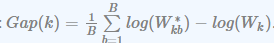
选择满足下式的最小的k:

R实现
datanovia教程是介绍了两个不同的R包,分别如下:
- factoextra
- NbClust
pkgs <- c("factoextra",  "NbClust")
install.packages(pkgs)

library(factoextra)
library(NbClust)
而我们之前的微信教程用的应该是另一个API实现的gap method。
factoextra的fviz_nbclust()函数
3 methods [elbow, silhouette and gap statistic]
for any partitioning clustering methods [K-means, K-medoids (PAM), CLARA, HCUT].
fviz_nbclust(x, FUNcluster, method = c("silhouette", "wss", "gap_stat"))
- x: numeric matrix or data frame
- FUNcluster: a partitioning function. Allowed values include kmeans, pam, clara and hcut (for hierarchical clustering).
- method: the method to be used for determining the optimal number of clusters. (注意wss代表elbow方法)
NbClust的NbClust() 函数
NbClust(data = NULL, diss = NULL, distance = "euclidean",
        min.nc = 2, max.nc = 15, method = NULL)
data: matrix
diss: dissimilarity matrix to be used. By default, diss=NULL, but if it is replaced by a dissimilarity matrix, distance should be “NULL”
distance: the distance measure to be used to compute the dissimilarity matrix. Possible values include “euclidean”, “manhattan” or “NULL”.
min.nc, max.nc: minimal and maximal number of clusters, respectively
method: The cluster analysis method to be used including “ward.D”, “ward.D2”, “single”, “complete”, “average”, “kmeans” and more.
微信中的那个函数
set.seed(123)
## Compute the gap statistic
gap_stat = clusGap(df, FUN = kmeans, nstart = 25, K.max = 10, B = 500)
# Plot the result
fviz_gap_stat(gap_stat)
顾名思义,就是用专门计算gap的函数,并画出来。按理说和
fviz_nbclust(x, FUNcluster, method = "gap_stat")是一样的。
聚类评估方法Cluster Validation
参考教程:datanovia的教程
首先分了三大类:
internal:只用聚类结果,不用任何别的信息(一般说的其实就是这种)
external:基本上是把聚类当分类,监督学习
relative:同一种聚类方法中改变参数,来判断。通常用于聚类个数的判断
那我们应该是一种介于internal和external之间的方法?
internal
两个总原则:
类内相似,类间不同 (Compactness & Separation)
基本原则都是用
(类间相异性/类内相似性) 或 (类间相异性-类内相似性)
轮廓系数(Silhouette coefficient)
- 每一个样本点都有一个轮廓系数
- a是这个点到本簇所有点的平均距离
- b是这个点到其他所有簇的平均距离的最小值
- 这个点的轮廓系数为(b-a)/max{a,b}.
- 因此轮廓系数自然处于-1~1之间。
- 越大越好。
- 如果是负的就很不好,说明到别的簇比到自己簇还近了。

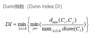
Dunn指数
分子:我簇和你簇的样本中,离得最近的,之间的距离。取最小值。
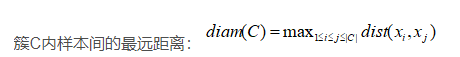
分母:我簇所有样本中,离得最远的,之间的距离,取最大值。

另一版本的描述更复杂,我个人还是选上面那个了。
external
暂时略
其他
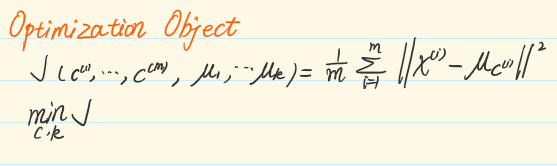
k means方法的目标函数
intra-cluster variation [or total within-cluster sum of square (WSS)]
簇内方差和。
total估计是求和,就不需要想下图这样除以m了。
R语言实现
The following R packages are required in this chapter:
- factoextra for data visualization
- fpc for computing clustering validation statistics
- NbClust for determining the optimal number of clusters in the data set.
# Install the packages:
install.packages(c("factoextra", "fpc", "NbClust"))
# Load the packages:
library(factoextra)
library(fpc)
library(NbClust)
绘制轮廓系数图
使用fviz_silhouette() [factoextra package]来绘制轮廓系数图silhouette coefficients:
#提取聚类轮廓图
sil = silhouette(km.res$cluster, dist(df))
#rownames(sil) = rownames(dataset)
#head(sil[, 1:3]) # 查看数据集前6行数据
# Visualize
fviz_silhouette(sil)
如果出现负轮廓系数,可以用一下代码打印其名字:
# Silhouette width of observation
sil <- km.res$silinfo$widths[, 1:3]
# Objects with negative silhouette
neg_sil_index <- which(sil[, 'sil_width'] < 0)
sil[neg_sil_index, , drop = FALSE]
计算各种指标
要用fpc包
internal可以使用
cluster.stats() [fpc package]
NbClust() [in NbClust package]
略去细节,详情看原文
external
如果要比较两种不同的cluster结果,有两种方法:
corrected Rand index &Meila’s VI.
其中第一种Rand index
Its range is -1 (no agreement) to 1 (perfect agreement).
计算方法如下:
library("fpc")
# Compute cluster stats
species <- as.numeric(iris$Species)
clust_stats <- cluster.stats(d = dist(df),
                             species, km.res$cluster)
# Corrected Rand index
clust_stats$corrected.rand
## [1] 0.62
# VI
clust_stats$vi
## [1] 0.748
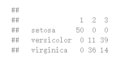
也直接用表格显示结果,首行是cluster1的标签,首列是cluster2的标签:
table(iris
S
p
e
c
i
e
s
,
k
m
.
r
e
s
Species, km.res
Species,km.rescluster)
选择聚类方法
用clValid包。
常见聚类方法包括:
K-means, K-medoids (PAM), CLARA, HCUT,hierarchical。
clValid包用两种评价指标:
internal measures: connectivity, 轮廓系数,Dunn,系数
stability measures: 每次移除一列,观察聚类结果的稳定性
Cluster stability measures include:
- The average proportion of non-overlap (APN)
- The average distance (AD)
- The average distance between means (ADM)
- The figure of merit (FOM)
clValid(obj, nClust, clMethods = "hierarchical",
        validation = "stability", maxitems = 600,
        metric = "euclidean", method = "average")
- obj: A numeric matrix or data frame. Rows are the items to be clustered and columns are samples.
- nClust: A numeric vector specifying the numbers of clusters to be evaluated. e.g., 2:10
- clMethods: The clustering method to be used. Available options are “hierarchical”, “kmeans”, “diana”, “fanny”, “som”, “model”, “sota”, “pam”, “clara”, and “agnes”, with multiple choices allowed.
- validation: The type of validation measures to be used. Allowed values are “internal”, “stability”, and “biological”, with multiple choices allowed.
- maxitems: The maximum number of items (rows in matrix) which can be clustered.
- metric: The metric used to determine the distance matrix. Possible choices are “euclidean”, “correlation”, and “manhattan”.
- method: For hierarchical clustering (hclust and agnes), the agglomeration method to be used. Available choices are “ward”, “single”, “complete” and “average”.
例子有点没看懂。后面实践一下再。
Computing P-value for Hierarchical Clustering
这个是针对hierarchical clustering的,应该先学一下hierarchical clustering再说。
其他相关课程
课程底下推荐了三个课:
PARTITIONAL CLUSTERING IN R: THE ESSENTIALS
HIERARCHICAL CLUSTERING IN R: THE ESSENTIALS
又在datanovia搜索了一下cluster 关键词,找到一堆。
发现下面这个就是我微信那篇的原文啊。。。
CLUSTER ANALYSIS IN R SIMPLIFIED AND ENHANCED
下面这个比较全面,从基础到高阶:
Cluster Analysis in R: Practical Guide


 1122
1122


 被折叠的 条评论
为什么被折叠?
被折叠的 条评论
为什么被折叠?
 到【灌水乐园】发言


