Lenet5网络结构详解及tensorflow实现

LeNet5特征能够总结为如下几点：

1）卷积神经网络使用三个层作为一个系列： 卷积，池化，非线性；

2） 使用卷积提取空间特征；

3）使用映射到空间均值下采样（subsample）；

4）双曲线（tanh）或S型（sigmoid）形式的非线性；

5）多层神经网络（MLP）作为最后的分类器；

6）层与层之间的稀疏连接矩阵避免大的计算成本；

CNN实现对mnist数据集的分类

import tensorflow as tf 
from tensorflow.examples.tutorials.mnist import input_data
 
mnist = input_data.read_data_sets("MNIST_data/",one_hot = True)
sess = tf.InteractiveSession()
 
def weight_variable(shape):
	initial = tf.truncated_normal(shape,stddev=0.1)
	return tf.Variable(initial)
 
def bias_variable(shape):
	initial = tf.constant(0.1,shape = shape)
	return tf.Variable(initial)
 
def conv2d(x,W):
	return tf.nn.conv2d(x,W,strides=[1,1,1,1],padding='SAME')
 
def max_pool_2x2(x):
	return tf.nn.max_pool(x,ksize=[1,2,2,1],strides=[1,2,2,1],padding='SAME')
 
x = tf.placeholder(tf.float32,[None,784])
y_ = tf.placeholder(tf.float32,[None,10])
x_image = tf.reshape(x,[-1,28,28,1])
 
# Conv1 Layer
W_conv1 = weight_variable([5,5,1,32])
b_conv1 = bias_variable([32])
h_conv1 = tf.nn.relu(conv2d(x_image,W_conv1) + b_conv1)
h_pool1 = max_pool_2x2(h_conv1)
 
# Conv2 Layer
W_conv2 = weight_variable([5,5,32,64])
b_conv2 = bias_variable([64])
h_conv2 = tf.nn.relu(conv2d(h_pool1,W_conv2) + b_conv2)
h_pool2 = max_pool_2x2(h_conv2)
 
W_fc1 = weight_variable([7*7*64,1024])
b_fc1 = bias_variable([1024])
h_pool2_flat = tf.reshape(h_pool2,[-1,7*7*64])
h_fc1 = tf.nn.relu(tf.matmul(h_pool2_flat,W_fc1) + b_fc1)
 
keep_prob = tf.placeholder(tf.float32)
h_fc1_drop = tf.nn.dropout(h_fc1,keep_prob)
 
W_fc2 = weight_variable([1024,10])
b_fc2 = bias_variable([10])
y_conv = tf.nn.softmax(tf.matmul(h_fc1_drop,W_fc2) + b_fc2)
 
cross_entropy = tf.reduce_mean(-tf.reduce_sum(y_ * tf.log(y_conv),reduction_indices=[1]))
train_step = tf.train.AdamOptimizer(1e-4).minimize(cross_entropy)
 
correct_prediction = tf.equal(tf.argmax(y_conv,1),tf.argmax(y_,1))
accuracy = tf.reduce_mean(tf.cast(correct_prediction,tf.float32))
 
tf.global_variables_initializer().run()
for i in range(20000):
	batch = mnist.train.next_batch(50)
	if i % 1000 == 0:
		train_accuracy = accuracy.eval(feed_dict={x:batch[0],y_:batch[1],keep_prob:1.0})
		print("step %d, training accuracy %g"%(i,train_accuracy))
	train_step.run(feed_dict={x:batch[0],y_:batch[1],keep_prob:0.5})
 
print("test accuracy %g"%accuracy.eval(feed_dict={x:mnist.test.images,y_:mnist.test.labels,keep_prob:1.0}))

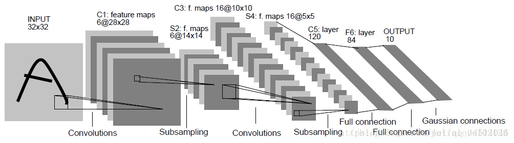
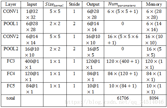
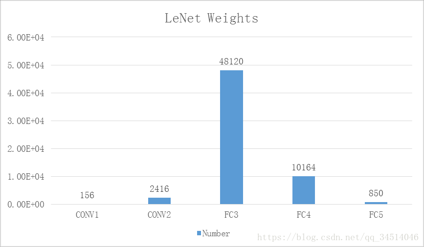
第一层，卷积层

这一层的输入就是原始的图像像素32*32*1。第一个卷积层过滤器尺寸为5*5，深度为6，不使用全0填充，步长为1。所以这一层的输出：28*28*6，卷积层共有5*5*1*6+6=156个参数

第二层，池化层

这一层的输入为第一层的输出，是一个28*28*6的节点矩阵。本层采用的过滤器大小为2*2，长和宽的步长均为2，所以本层的输出矩阵大小为14*14*6。

第三层，卷积层

本层的输入矩阵大小为14*14*6，使用的过滤器大小为5*5，深度为16.本层不使用全0填充，步长为1。本层的输出矩阵大小为10*10*16。本层有5*5*6*16+16=2416个参数。

第四层，池化层

本层的输入矩阵大小10*10*16。本层采用的过滤器大小为2*2，长和宽的步长均为2，所以本层的输出矩阵大小为5*5*16。

第五层，全连接层

本层的输入矩阵大小为5*5*16，在LeNet-5论文中将这一层成为卷积层，但是因为过滤器的大小就是5*5，所以和全连接层没有区别。如果将5*5*16矩阵中的节点拉成一个向量，那么这一层和全连接层就一样了。本层的输出节点个数为120，总共有5*5*16*120+120=48120个参数。

第六层，全连接层

本层的输入节点个数为120个，输出节点个数为84个，总共参数为120*84+84=10164个。

第七层，全连接层

本层的输入节点个数为84个，输出节点个数为10个，总共参数为84*10+10=850

Tensorflow实现LeNet-5

LeNet_inference.py

# _*_ coding: utf-8 _*_
import tensorflow as tf

# 配置神经网络的参数
INPUT_NODE = 784
OUTPUT_NODE = 10

IMAGE_SIZE = 28
NUM_CHANNELS = 1
NUM_LABELS = 10

# 第一个卷积层的尺寸和深度
CONV1_DEEP = 32
CONV1_SIZE = 5
# 第二个卷积层的尺寸和深度
CONV2_DEEP = 64
CONV2_SIZE = 5
# 全连接层的节点个数
FC_SIZE = 512

# 定义卷积神经网络的前向传播过程。这里添加了一个新的参数train，用于区别训练过程和测试过程。在这个程序中将用到dropout方法
# dropout可以进一步提升模型可靠性并防止过拟合（dropout过程只在训练时使用）
def inference(input_tensor, train, regularizer):
    with tf.variable_scope('layer1-conv1'):
        conv1_weights = tf.get_variable('weight', [CONV1_SIZE, CONV1_SIZE, NUM_CHANNELS, CONV1_DEEP],
                                        initializer=tf.truncated_normal_initializer(stddev=0.1))
        conv1_biases = tf.get_variable('bias', [CONV1_DEEP],
                                       initializer=tf.constant_initializer(0.0))
        conv1 = tf.nn.conv2d(input_tensor, conv1_weights, strides=[1, 1, 1, 1], padding='SAME')
        relu1 = tf.nn.relu(tf.nn.bias_add(conv1, conv1_biases))

    with tf.name_scope('layer2-pool1'):
        pool1 = tf.nn.max_pool(relu1, ksize=[1, 2, 2, 1], strides=[1, 2, 2, 1], padding='SAME')

    with tf.variable_scope('layer3-conv2'):
        conv2_weights = tf.get_variable('weight', [CONV2_SIZE, CONV2_SIZE, CONV1_DEEP, CONV2_DEEP],
                                        initializer=tf.truncated_normal_initializer(stddev=0.1))
        conv2_biases = tf.get_variable('bias', [CONV2_DEEP],
                                       initializer=tf.constant_initializer(0.0))
        conv2 = tf.nn.conv2d(pool1,conv2_weights, strides=[1, 1, 1, 1], padding='SAME')
        relu2 = tf.nn.relu(tf.nn.bias_add(conv2, conv2_biases))

    with tf.name_scope('layer4-pool2'):
        pool2 = tf.nn.max_pool(relu2, ksize=[1, 2, 2, 1], strides=[1, 2, 2, 1], padding='SAME')

    pool2_shape = pool2.get_shape().as_list()
    nodes = pool2_shape[1] * pool2_shape[2] * pool2_shape[3]

    reshaped = tf.reshape(pool2, [pool2_shape[0], nodes])

    with tf.variable_scope('layer5-fc1'):
        fc1_weights = tf.get_variable('weight', [nodes, FC_SIZE],
                                      initializer=tf.truncated_normal_initializer(stddev=0.1))
        if regularizer != None:
            tf.add_to_collection('losses', regularizer(fc1_weights))
        fc1_biases = tf.get_variable('bias', [FC_SIZE],
                                     initializer=tf.constant_initializer(0.0))
        fc1 = tf.nn.relu(tf.matmul(reshaped, fc1_weights) + fc1_biases)
        if train:
            fc1 = tf.nn.dropout(fc1, 0.5)

    with tf.variable_scope('layer6-fc2'):
        fc2_weights = tf.get_variable('weight', [FC_SIZE, NUM_LABELS],
                                      initializer=tf.truncated_normal_initializer(stddev=0.1))
        if regularizer != None:
            tf.add_to_collection('losses', regularizer(fc2_weights))
        fc2_biases = tf.get_variable('bias', [NUM_LABELS],
                                     initializer=tf.constant_initializer(0.0))
        logit = tf.matmul(fc1, fc2_weights) + fc2_biases

    return logit

LeNet_train.py

# _*_ coding: utf-8 _*_
import os

import tensorflow as tf
import numpy as np
from tensorflow.examples.tutorials.mnist import input_data

# 加载mnist_inference.py中定义的常量和前向传播的函数
import LeNet_inference

# 配置神经网络的参数
BATCH_SIZE = 100
LEARNING_RATE_BASE = 0.8
LEARNING_RATE_DECAY = 0.99
REGULARAZTION_RATE = 0.0001
TRAIN_STEPS = 30000
MOVING_AVERAGE_DECAY = 0.99

MODEL_SAVE_PATH = "./model/"
MODEL_NAME = "model3.ckpt"

def train(mnist):
    x = tf.placeholder(tf.float32, [BATCH_SIZE, LeNet_inference.IMAGE_SIZE,
                                    LeNet_inference.IMAGE_SIZE,
                                    LeNet_inference.NUM_CHANNELS], name='x-input')
    y_ = tf.placeholder(tf.float32, [None, LeNet_inference.OUTPUT_NODE], name='y-input')

    regularizer = tf.contrib.layers.l2_regularizer(REGULARAZTION_RATE)

    y = LeNet_inference.inference(x, train, regularizer)

    global_step = tf.Variable(0, trainable=False)

    variable_average = tf.train.ExponentialMovingAverage(MOVING_AVERAGE_DECAY, global_step)
    variable_average_op = variable_average.apply(
        tf.trainable_variables())
    cross_entropy = tf.nn.sparse_softmax_cross_entropy_with_logits(labels=tf.argmax(y_, 1), logits=y)
    cross_entropy_mean = tf.reduce_mean(cross_entropy)

    loss = cross_entropy_mean + tf.add_n(tf.get_collection('losses'))

    learning_rate = tf.train.exponential_decay(LEARNING_RATE_BASE,
                                               global_step=global_step, decay_steps=mnist.train.num_examples / BATCH_SIZE,
                                               decay_rate=LEARNING_RATE_DECAY)
    train_step = tf.train.GradientDescentOptimizer(learning_rate).minimize(loss, global_step=global_step)

    with tf.control_dependencies([train_step, variable_average_op]):
        train_op = tf.no_op(name='train')

    saver = tf.train.Saver()
    with tf.Session() as sess:
        tf.global_variables_initializer().run()

        for i in range(TRAIN_STEPS):
            xs, ys = mnist.train.next_batch(BATCH_SIZE)
            xs = np.reshape(xs, [BATCH_SIZE, LeNet_inference.IMAGE_SIZE,
                                    LeNet_inference.IMAGE_SIZE,
                                    LeNet_inference.NUM_CHANNELS])
            _, loss_value, step = sess.run([train_op, loss, global_step], feed_dict={x: xs, y_: ys})
            if i % 1000 == 0:
                print("After %d training steps, loss on training"
                      "batch is %g" % (step, loss_value))
                saver.save(sess, os.path.join(MODEL_SAVE_PATH, MODEL_NAME), global_step=global_step)

def main(argv=None):
    mnist = input_data.read_data_sets("E:\科研\TensorFlow教程\MNIST_data", one_hot=True)
    train(mnist)

if __name__ == '__main__':
    tf.app.run()

 

如何设计卷积神经网络架构

下面的正则化公式总结了一些经典的用于图片分类问题的卷积神经网络架构： 

输入层→（卷积层+→池化层？）+→全连接层+

“+”表示一层或多层，“？”表示有或者没有 

如何设置卷积层或池化层配置

• 过滤器的尺寸：1或3或5，有些网络中有过7甚至11
• 过滤器的深度：逐层递增。每经过一次池化层之后，卷积层深度*2
• 卷积层的步长：一般为1，有些也会使用2甚至3
• 池化层：最多的是max_pooling，过滤器边长一般为2或者3，步长一般为2或3