


朴素贝叶斯(naive bayes)法是基于贝叶斯定理与特征条件独立假设的分类方法。
- 优点:在数据较少的情况下仍然有效,可以处理多分类问题。
- 缺点:对入输入数据的准备方式较为敏感。
- 使用数据类型:标称型数据。
下面从一个简单问题出发,介绍怎么使用朴素贝叶斯解决分类问题。
一天,老师问了个问题,只根据头发和声音怎么判断一位同学的性别。
为了解决这个问题,同学们马上简单的统计了7位同学的相关特征,数据如下:
| 头发 | 声音 | 性别 |
|---|---|---|
| 长 | 粗 | 男 |
| 短 | 粗 | 男 |
| 短 | 粗 | 男 |
| 长 | 细 | 女 |
| 短 | 细 | 女 |
| 短 | 粗 | 女 |
| 长 | 粗 | 女 |
| 长 | 粗 | 女 |
这个问题之前用决策树做过了,这里我们换一种思路。
要是知道男生和女生头发长短的概率以及声音粗细的概率,我们就可以计算出各种情况的概率,然后比较概率大小,来判断性别。
假设抽样样本足够大,我们可以近似认为可以代表所有数据,假设上位7位同学能代表所有数据,这里方便计算~
由这7位同学,我们马上得出下面表格概率分布。
| 性别 | 头发长 | 声音粗 |
|---|---|---|
| 男 | 1/3 | 1 |
| 女 | 3/5 | 3/5 |
假设头发和声音都是独立特征,于是
男生头发长声音粗的概率=3/8*1/3*1=1/8
女生头发长声音粗的概率=5/8*3/5*3/5=9/40
因为1/8<9/40所以如果一个人,头发长,声音粗,那么这个人更可能是女生,于是出现这些特征就是女生。其他特征依次类推。
这就是朴素贝叶斯分类方法。是的,就是这么简单。
下面来解释原理,先看贝叶斯公式:

公式中,事件Bi的概率为P(Bi),事件Bi已发生条件下事件A的概率为P(A│Bi),事件A发生条件下事件Bi的概率为P(Bi│A)。
带入我们的例子中,判断头发长的人性别:
P(男|头发长)=P(头发长|男)*P(男)/P(头发长)
P(女|头发长)=P(头发长|女)*P(女)/P(头发长)
判断头发长、声音粗的人性别:
P(男|头发长声音粗)=P(头发长|男)P(声音粗|男)*P(男)/P(头发长声音粗)
P(女|头发长声音粗)=P(头发长|女)P(声音粗|女)*P(女)/P(头发长声音粗)
可以看到,比较最后比较概率,只用比较分子即可。也就是前面计算头发长声音粗的人是男生女生的概率。
下面应用于文本分类,文本分类不想上面例子有具体的特征,需先建立文本特征。以下为文本分类的一个简单例子。
# _*_ coding:utf-8 _*_
from numpy import *
import re
import random

def loadDataSet(): #创建样例数据
    postingList = [['my', 'dog', 'has', 'flea', 'problems', 'help', 'please'],
                   ['maybe', 'not', 'take', 'him', 'to', 'dog', 'park', 'stupid'],
                   ['my', 'dalmation', 'is', 'so', 'cute', 'I', 'love', 'him'],
                   ['stop', 'posting', 'stupid', 'worthless', 'garbage'],
                   ['mr', 'licks', 'ate', 'my', 'steak', 'how', 'to', 'stop', 'him'],
                   ['quit', 'buying', 'worthless', 'dog', 'food', 'stupid']]
    classVec = [0, 1, 0, 1, 0, 1]  #1代表脏话
    return postingList, classVec

def createVocabList(dataSet):  #创建词库 这里就是直接把所有词去重后,当作词库
    vocabSet = set([])
    for document in dataSet:
        vocabSet = vocabSet | set(document)
    return list(vocabSet)

def setOfWords2Vec(vocabList, inputSet):  #文本词向量。词库中每个词当作一个特征,文本中就该词,该词特征就是1,没有就是0
    returnVec = [0] * len(vocabList)
    for word in inputSet:
        if word in vocabList:
            returnVec[vocabList.index(word)] = 1
        else:
            print("the word: %s is not in my Vocabulary!" % word)
    return returnVec


def trainNB0(trainMatrix, trainCategory):
    numTrainDocs = len(trainMatrix)
    numWords = len(trainMatrix[0])
    pAbusive = sum(trainCategory) / float(numTrainDocs)
    p0Num = ones(numWords) #防止某个类别计算出的概率为0,导致最后相乘都为0,所以初始词都赋值1,分母赋值为2.
    p1Num = ones(numWords)
    p0Denom = 2
    p1Denom = 2
    for i in range(numTrainDocs):
        if trainCategory[i] == 1:
            p1Num += trainMatrix[i]
            p1Denom += sum(trainMatrix[i])
        else:
            p0Num += trainMatrix[i]
            p0Denom += sum(trainMatrix[i])
    p1Vect = log(p1Num / p1Denom)  #这里使用了Log函数,方便计算,因为最后是比较大小,所有对结果没有影响。
    p0Vect = log(p0Num / p0Denom)
    return p0Vect, p1Vect, pAbusive

def classifyNB(vec2Classify,p0Vec,p1Vec,pClass1): #比较概率大小进行判断,
    p1 = sum(vec2Classify*p1Vec)+log(pClass1)
    p0 = sum(vec2Classify*p0Vec)+log(1-pClass1)
    if p1>p0:
        return 1
    else:
        return 0

def testingNB():
    listOPosts,listClasses = loadDataSet()
    myVocabList = createVocabList(listOPosts)
    trainMat=[]
    for postinDoc in listOPosts:
        trainMat.append(setOfWords2Vec(myVocabList, postinDoc))
    p0V,p1V,pAb = trainNB0(array(trainMat),array(listClasses))
    testEntry = ['love', 'my', 'dalmation'] # 测试数据
    thisDoc = array(setOfWords2Vec(myVocabList, testEntry))
    print(testEntry,'classified as: ',classifyNB(thisDoc,p0V,p1V,pAb))
    testEntry = ['stupid', 'garbage'] # 测试数据
    thisDoc = array(setOfWords2Vec(myVocabList, testEntry))
    print(testEntry,'classified as: ',classifyNB(thisDoc,p0V,p1V,pAb))

if __name__=='__main__':
    testingNB()
- 1
- 2
- 3
- 4
- 5
- 6
- 7
- 8
- 9
- 10
- 11
- 12
- 13
- 14
- 15
- 16
- 17
- 18
- 19
- 20
- 21
- 22
- 23
- 24
- 25
- 26
- 27
- 28
- 29
- 30
- 31
- 32
- 33
- 34
- 35
- 36
- 37
- 38
- 39
- 40
- 41
- 42
- 43
- 44
- 45
- 46
- 47
- 48
- 49
- 50
- 51
- 52
- 53
- 54
- 55
- 56
- 57
- 58
- 59
- 60
- 61
- 62
- 63
- 64
- 65
- 66
- 67
- 68
- 69
- 70
- 71
- 72
- 73
- 74
#输出结果
['love', 'my', 'dalmation'] classified as:  0
['stupid', 'garbage'] classified as:  1
- 1
- 2
- 3
参考:
- Machine Learning in Action
- 统计学习方法
Svm(support Vector Mac)又称为支持向量机,是一种二分类的模型。当然如果进行修改之后也是可以用于多类别问题的分类。支持向量机可以分为线性核非线性两大类。其主要思想为找到空间中的一个更够将所有数据样本划开的超平面,并且使得本本集中所有数据到这个超平面的距离最短。
一、基于最大间隔分隔数据
1.1支持向量与超平面
在了解svm算法之前,我们首先需要了解一下线性分类器这个概念。比如给定一系列的数据样本,每个样本都有对应的一个标签。为了使得描述更加直观,我们采用二维平面进行解释,高维空间原理也是一样。举个简单子:如下图所示是一个二维平面,平面上有两类不同的数据,分别用圆圈和方块表示。我们可以很简单地找到一条直线使得两类数据正好能够完全分开。但是能将据点完全划开直线不止一条,那么在如此众多的直线中我们应该选择哪一条呢?从直观感觉上看图中的几条直线, 是不是要更好一些呢?是的我们就是希望寻找到这样的直线,使得距离这条直线最近的点到这条直线的距离最短。这读起来有些拗口,我们从图三中直观来解释这一句话就是要求的两条外面的线之间的间隔最大。这是可以理解的,因为假如数据样本是随机出现的,那么这样分割之后数据点落入到其类别一侧的概率越高那么最终预测的准确率也会越高。在高维空间中这样的直线称之为超平面,因为当维数大于三的时候我们已经无法想象出这个平面的具体样子。那些距离这个超平面最近的点就是所谓支持向量,实际上如果确定了支持向量也就确定了这个超平面,找到这些支持向量之后其他样本就不会起作用了。

图 1 图2
1.2寻找最大间隔
1.2.1点到超平面的距离公式
既然这样的直线是存在的,那么我们怎样寻找出这样的直线呢?与二维空间类似,超平面的方程也可以写成一下形式:
 (1.1)
(1.1)
有了超平面的表达式之后之后,我们就可以计算样本点到平面的距离了。假设 为样本的中的一个点,其中
 表示为第个特征变量。那么该点到超平面的距离
 就可以用如下公式进行计算:
 (1.2)
(1.2)
其中||W||为超平面的范数,常数b类似于直线方程中的截距。
上面的公式可以利用解析几何或高中平面几何知识进行推导,这里不做进一步解释。
1.2.2最大间隔的优化模型
现在我们已经知道了如何去求数据点到超平面的距离,在超平面确定的情况下,我们就能够找出所有支持向量,然后计算出间隔margin。每一个超平面都对应着一个margin,我们的目标就是找出所有margin中最大的那个值对应的超平面。因此用数学语言描述就是确定w、b使得margin最大。这是一个优化问题其目标函数可以写成:
 (1.3)
(1.3)
其中 表示数据点的标签,且其为-1或1。距离用
 计算,这是就能体会出-1和1的好处了。如果数据点在平面的正方向(即+1类)那么是一个正数,而当数据点在平面的负方向时(即-1类),依然是一个正数,这样就能够保证始终大于零了。注意到当w和b等比例放大时,d的结果是不会改变的。因此我们可以令所有支持向量的u为1,而其他点的u大1这是可以办通过调节w和b求到的。因此上面的问题可以简化为:
  (1.4)
(1.4)
为了后面计算的方便,我们将目标函数等价替换为:
 (1.5)
(1.5)
这是一个有约束条件的优化问题,通常我们可以用拉格朗日乘子法来求解。拉格朗日乘子法的介绍可以参考这篇博客。应用拉格朗日乘子法如下:
令  (1.6)
(1.6)
求L关于求偏导数得: (1.7)
(1.7)
将(1.7)代入到(1.6)中化简得:
 (1.8)
(1.8)
原问题的对偶问题为:
 (1.9)
(1.9)
该对偶问题的KKT条件为
 (1.10)
到此,似乎问题就能够完美地解决了。但是这里有个假设:数据必须是百分之百可分的。但是实际中的数据几乎都不那么“干净”,或多或少都会存在一些噪点。为此下面我们将引入了松弛变量来解决这种问题。
1.2.3松弛变量
由上一节的分析我们知道实际中很多样本数据都不能够用一个超平面把数据完全分开。如果数据集中存在噪点的话,那么在求超平的时候就会出现很大问题。从图三中课看出其中一个蓝点偏差太大,如果把它作为支持向量的话所求出来的margin就会比不算入它时要小得多。更糟糕的情况是如果这个蓝点落在了红点之间那么就找不出超平面了。
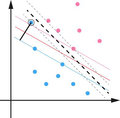
图 3
因此引入一个松弛变量ξ来允许一些数据可以处于分隔面错误的一侧。这时新的约束条件变为:
 (1.11)
式中ξi的含义为允许第i个数据点允许偏离的间隔。如果让ξ任意大的话,那么任意的超平面都是符合条件的了。所以在原有目标的基础之上,我们也尽可能的让ξ的总量也尽可能地小。所以新的目标函数变为:
 (1.12)
 (1.13)
其中的C是用于控制“最大化间隔”和“保证大部分的点的函数间隔都小于1”这两个目标的权重。将上述模型完整的写下来就是:
 (1.14)
新的拉格朗日函数变为:
 (1.15)
接下来将拉格朗日函数转化为其对偶函数,首先对 分别求
分别求 ξ的偏导,并令其为0,结果如下:
 (1.16)
代入原式化简之后得到和原来一样的目标函数:
 (1.17)
但是由于我们得到 而
而 ,因此有
,因此有 所以对偶问题写成:
 (1.18)
经过添加松弛变量的方法,我们现在能够解决数据更加混乱的问题。通过修改参数C,我们可以得到不同的结果而C的大小到底取多少比较合适,需要根据实际问题进行调节。
1.2.4核函数
以上讨论的都是在线性可分情况进行讨论的,但是实际问题中给出的数据并不是都是线性可分的,比如有些数据可能是如图4样子。 
图4
那么这种非线性可分的数据是否就不能用svm算法来求解呢?答案是否定的。事实上,对于低维平面内不可分的数据,放在一个高维空间中去就有可能变得可分。以二维平面的数据为例,我们可以通过找到一个映射将二维平面的点放到三维平面之中。理论上任意的数据样本都能够找到一个合适的映射使得这些在低维空间不能划分的样本到高维空间中之后能够线性可分。我们再来看一下之前的目标函数:
 (1.19)
定义一个映射使得将所有映射到更高维空间之后等价于求解上述问题的对偶问题:
 (1.20)
这样对于线性不可分的问题就解决了,现在只需要找出一个合适的映射即可。当特征变量非常多的时候在,高维空间中计算内积的运算量是非常庞大的。考虑到我们的目的并不是为找到这样一个映射而是为了计算其在高维空间的内积,因此如果我们能够找到计算高维空间下内积的公式,那么就能够避免这样庞大的计算量,我们的问题也就解决了。实际上这就是我们要找的核函数 ,即两个向量在隐式映射后的空间中的内积。下面的一个简单例子可以帮助我们更好地理解核函数。
通过以上例子,我们可以很明显地看到核函数是怎样运作的。上述问题的对偶问题可以写成如下形式:
 (1.21)
那么怎样的函数才可以作为核函数呢?下面的一个定理可以帮助我们判断。
Mercer定理:任何半正定的函数都可以作为核函数。其中所谓半正定函数 是指拥有训练集数据集合,我们定义一个矩阵的元素
 ,这个矩阵是
 的矩阵,如果这个矩阵是半正定的,那么
 就称为半正定函数。
值得注意的是,上述定理中所给出的条件是充分条件而非充要条件。因为有些非正定函数也可以作为核函数。
下面是一些常用的核函数:
表1 常用核函数表
核函数名称 | 核函数表达式 | 核函数名称 | 核函数表达式 |
线性核 |
| 指数核 |
|
多项式核 |
| 拉普拉斯核 |
|
高斯核 |
| Sigmoid核 |
|


现在我们已经了解了一些支持向量机的理论基础,我们通过对偶问题的的转化将最开始求 的问题转化为求
 的对偶问题。只要找到所有的(即找出所有支持向量),我们就能够确定
 。然后就可以通过计算数据点到这个超平面的距离从而判断出该数据点的类别。
二、Smo算法原理
2.1 约束条件
根据以上问题的分析,我们已经将原始问题转化为了求的值,即求下面优化模型的解:
 (2.1)
(2.1)
求解的值的方法有很多,Smo算法就是其中一种比较常用的方法。该算法是由John Platt在1996年发布,他的思路是将大的优化问题转化为小的优化问题。而这些小的优化问题往往更容易求解,并且对它们进行顺序求解的结果和将它们作为整体求解的结果完全一致但是Smo算法的时间要小得多。
Smo算法的原理为:每次任意抽取两个乘子 和,
和, 然后固定和以外的其它乘子
 ,使得目标函数只是关于和的函数。然后增大其中一个乘子同时减少另外一个。这样,不断的从一堆乘子中任意抽取两个求解,不断的迭代求解子问题,最终达到求解原问题的目的。
而原对偶问题的子问题的目标函数可以表达成:
 (2.2)
(2.2)
其中:
 (2.3)
(2.3)
这里之所以算两个是因为 的限制,如果只改变其中的一个量,那么这个约束条件可能就不成立了。要解决这个问题,我们必须得选取这样的两个乘子。那么怎样确定这样的和呢?这是我们首先要考虑的问题,在《机器学习实战》这本书中,作者首先给出了一种简化版的方法,遍历每一个然后在剩余的中随机选取一个进行优化。虽然样也能够解决问题,但是运算量太大,因此考虑找一种更好的方法来寻找对。
为了表述方便,定义一个特征到输出结果的输出函数:
 (2.4)
(2.4)
该对偶问题中KKT条件为:
 (2.5)
(2.5)
根据上述问题的KKT条件可以得出目标函数中的的 含义如下:
含义如下:
1、  ,表明是正常分类,在边界外;
2、 ,表明是支持向量,在边界上;
3、 ,表明在两边界之间。
最优解需要满足KKT条件,因此需要满足以上的三个条件都满足。而不满足这三个条件的情况也有三种:
1、 <=1但是<C则是不满足的,而原本=C;
2、>=1但是>0则是不满足的,而原本=0;
3、=1但是=0或者=C则表明不满足的,而原本应该是0<<C.
也就是说如果存在不满足这些KKT条件的,我们就要更新它,这就是约束条件之一。其次,还受到约束条件 的限制,因此假设选择的两个因子为和,他们在更新前分别为
 在更新后为
在更新后为 ,为了保证上述约束条件成立必须要保证下列等式的成立:
 (2.6)
(2.6)
其中 为常数。
为常数。
2.2参数优化
因为两个因子不好同时求解,所以可先求第二个乘子 的解
的解 ,然后再用的解表示
 的解
的解 。为了求解,得先确定的取值范围。假设它的上下边界分别为H和L,那么有:
 (2.6)
(2.6)
接下来,综合 和
和 这两个约束条件,求取的取值范围。
当 时,根据
时,根据 可得
可得 ,所以有
,所以有 。
。
当 时,同样根据
 可得:
可得: ,所以有
,所以有 。
。
回顾第二个约束条件 : (2.7)
(2.7)
令其两边同时乘y1,可得:
 . (2.8)
其中: .
.
因此 可以用
可以用 表示,即:
表示,即:  (2.9)
(2.9)
令  (2.10)
经过转化之后可得:
 ,
, . (2.11)
那么如何来选择乘子 呢?对于第一个乘子,我们可以按照3种不满足KTT的条件来寻找。对于第二个乘子,我们可以寻找满足条件
 的乘子。
的乘子。
而b在满足以下条件时需要更新:
 (2.12)
且更新后的和如下:
 (2.13)
每次更新完两个乘子之后,都需要重新计算b以及对应的E。最后更新完所有的 ,y和b,这样模型也就出来了,从而可以计算出开始所说的分类函数:
 (2.14)
三、Svm的python实现与应用
第二节已经对Smo算法进行了充分的说明并进行了推导,现在一切都准备好了。接下来需要做的就是实现这些算法了,这里我参考了《机器学习实战》这本书中的代码,并利用该程序对一个问题进行了求解。由于代码数量过大,因此这里就不再列出,而是放在附录中。有兴趣的朋友可以直接下载,也可以去官网下载源代码。笔者在读这些代码的过程中,也遇到了许多困难,大部分都根据自己的情况进行了注释。
3.1问题描述
这里我选取的一个数据集为声呐数据集,该问题为需要根据声呐从不同角度返回的声音强度来预测被测物体是岩石还是矿井。数据集中共有208个数据,60个输入变量和1个输出变量。每个数据的前60个元素为不同方向返回的声音强度,最后一个元素为本次用于声呐测试的物体类型。其中标签M表示矿井,标签R为岩石。
3.2数据预处理
所给数据中没有缺失值和异常值,因此不需要对数据集进行清洗。注意到所给数据集的标签为字母类型,而svm算法的标准标签为“-1”和“1”的形式,所以需要对标签进行转化,用“-1”、“1”分别代替M和R。由于该数据集中所给标签相同的数据都放在了一起,因此先对数据顺序进行了打乱。代码如下:
def loadDataSet(fileName): dataMat=[];labelMat=[];data=[] fr=open(fileName) for line in fr.readlines(): line=line.replace(',','\t')#去除逗号 line=line.replace('M','-1')#对标签进行替换 line=line.replace('R','1') lineArr=line.strip('\n').split('\t')#分割数据 data.append([float(lineArr[i]) for i in range(len(lineArr))]) random.shuffle(data) #随机打乱列表 for i in range(len(data)): dataMat.append(data[i][0:len(data)-1]) labelMat.append(data[i][-1]) return dataMat,labelMat |
3.3模型训练及测试
首先测试了一下将所有数据即作为训练集又作为测试集,然后用Smo模型进行训练找到所有的支持向量。最后根据训练好的模型进行求解,最终测试的准确率平均为54%。如果把数据集分成测试集和训练集,发现测试的准确率也在这附近。而根据网上数据统计该数据集测试的准确率最高为84%,一般情况下为百分之六十几。数据集本身是造成测试准确率低的一个原因,但是另外一个更加重要的原因大概是参数的选择问题。如何选取合适的参数是一个值得思考的问题,在接下来的学习过程中我也会注意一下参数选取这个问题。到这里,关于svm的算法就告一段落了。
-
#svm算法的实现
-
from numpy
import*
-
import random
-
from time
import*
-
def loadDataSet(fileName):
#输出dataArr(m*n),labelArr(1*m)其中m为数据集的个数
-
dataMat=[];labelMat=[]
-
fr=open(fileName)
-
for line
in fr.readlines():
-
lineArr=line.strip().split(
'\t')
#去除制表符,将数据分开
-
dataMat.append([float(lineArr[
0]),float(lineArr[
1])])
#数组矩阵
-
labelMat.append(float(lineArr[
2]))
#标签
-
return dataMat,labelMat
-
-
def selectJrand(i,m):
#随机找一个和i不同的j
-
j=i
-
while(j==i):
-
j=int(random.uniform(
0,m))
-
return j
-
-
def clipAlpha(aj,H,L):
#调整大于H或小于L的alpha的值
-
if aj>H:
-
aj=H
-
if aj<L:
-
aj=L
-
return aj
-
-
def smoSimple(dataMatIn,classLabels,C,toler,maxIter):
-
dataMatrix=mat(dataMatIn);labelMat=mat(classLabels).transpose()
#转置
-
b=
0;m,n=shape(dataMatrix)
#m为输入数据的个数,n为输入向量的维数
-
alpha=mat(zeros((m,
1)))
#初始化参数,确定m个alpha
-
iter=
0
#用于计算迭代次数
-
while (iter<maxIter):
#当迭代次数小于最大迭代次数时(外循环)
-
alphaPairsChanged=
0
#初始化alpha的改变量为0
-
for i
in range(m):
#内循环
-
fXi=float(multiply(alpha,labelMat).T*\
-
(dataMatrix*dataMatrix[i,:].T))+b
#计算f(xi)
-
Ei=fXi-float(labelMat[i])
#计算f(xi)与标签之间的误差
-
if ((labelMat[i]*Ei<-toler)
and(alpha[i]<C))
or\
-
((labelMat[i]*Ei>toler)
and(alpha[i]>
0)):
#如果可以进行优化
-
j=selectJrand(i,m)
#随机选择一个j与i配对
-
fXj=float(multiply(alpha,labelMat).T*\
-
(dataMatrix*dataMatrix[j,:].T))+b
#计算f(xj)
-
Ej=fXj-float(labelMat[j])
#计算j的误差
-
alphaIold=alpha[i].copy()
#保存原来的alpha(i)
-
alphaJold=alpha[j].copy()
-
if(labelMat[i]!=labelMat[j]):
#保证alpha在0到c之间
-
L=max(
0,alpha[j]-alpha[i])
-
H=min(C,C+alpha[j]-alpha[i])
-
else:
-
L=max(
0,alpha[j]+alpha[i]-C)
-
H=min(C,alpha[j]+alpha[i])
-
if L==H:print(
'L=H');
continue
-
eta=
2*dataMatrix[i,:]*dataMatrix[j,:].T-\
-
dataMatrix[i,:]*dataMatrix[i,:].T-\
-
dataMatrix[j,:]*dataMatrix[j,:].T
-
if eta>=
0:print(
'eta=0');
continue
-
alpha[j]-=labelMat[j]*(Ei-Ej)/eta
-
alpha[j]=clipAlpha(alpha[j],H,L)
#调整大于H或小于L的alpha
-
if (abs(alpha[j]-alphaJold)<
0.0001):
-
print(
'j not move enough');
continue
-
alpha[i]+=labelMat[j]*labelMat[i]*(alphaJold-alpha[j])
-
b1=b-Ei-labelMat[i]*(alpha[i]-alphaIold)*\
-
dataMatrix[i,:]*dataMatrix[i,:].T-\
-
labelMat[j]*(alpha[j]-alphaJold)*\
-
dataMatrix[i,:]*dataMatrix[j,:].T
#设置b
-
b2=b-Ej-labelMat[i]*(alpha[i]-alphaIold)*\
-
dataMatrix[i,:]*dataMatrix[i,:].T-\
-
labelMat[j]*(alpha[j]-alphaJold)*\
-
dataMatrix[j,:]*dataMatrix[j,:].T
-
if (
0<alpha[i])
and(C>alpha[j]):b=b1
-
elif(
0<alpha[j])
and(C>alpha[j]):b=b2
-
else:b=(b1+b2)/
2
-
alphaPairsChanged+=
1
-
print(
'iter:%d i:%d,pairs changed%d'%(iter,i,alphaPairsChanged))
-
if (alphaPairsChanged==
0):iter+=
1
-
else:iter=
0
-
print(
'iteraction number:%d'%iter)
-
return b,alpha
-
#定义径向基函数
-
def kernelTrans(X, A, kTup):
#定义核转换函数(径向基函数)
-
m,n = shape(X)
-
K = mat(zeros((m,
1)))
-
if kTup[
0]==
'lin': K = X * A.T
#线性核K为m*1的矩阵
-
elif kTup[
0]==
'rbf':
-
for j
in range(m):
-
deltaRow = X[j,:] - A
-
K[j] = deltaRow*deltaRow.T
-
K = exp(K/(
-1*kTup[
1]**
2))
#divide in NumPy is element-wise not matrix like Matlab
-
else:
raise NameError(
'Houston We Have a Problem -- \
-
That Kernel is not recognized')
-
return K
-
-
class optStruct:
-
def __init__(self,dataMatIn, classLabels, C, toler, kTup):
# Initialize the structure with the parameters
-
self.X = dataMatIn
-
self.labelMat = classLabels
-
self.C = C
-
self.tol = toler
-
self.m = shape(dataMatIn)[
0]
-
self.alphas = mat(zeros((self.m,
1)))
-
self.b =
0
-
self.eCache = mat(zeros((self.m,
2)))
#first column is valid flag
-
self.K = mat(zeros((self.m,self.m)))
-
for i
in range(self.m):
-
self.K[:,i] = kernelTrans(self.X, self.X[i,:], kTup)
-
-
def calcEk(oS, k):
-
fXk = float(multiply(oS.alphas,oS.labelMat).T*oS.K[:,k] + oS.b)
-
Ek = fXk - float(oS.labelMat[k])
-
return Ek
-
-
def selectJ(i, oS, Ei):
-
maxK =
-1; maxDeltaE =
0; Ej =
0
-
oS.eCache[i] = [
1,Ei]
-
validEcacheList = nonzero(oS.eCache[:,
0].A)[
0]
-
if (len(validEcacheList)) >
1:
-
for k
in validEcacheList:
#loop through valid Ecache values and find the one that maximizes delta E
-
if k == i:
continue
#don't calc for i, waste of time
-
Ek = calcEk(oS, k)
-
deltaE = abs(Ei - Ek)
-
if (deltaE > maxDeltaE):
-
maxK = k; maxDeltaE = deltaE; Ej = Ek
-
return maxK, Ej
-
else:
#in this case (first time around) we don't have any valid eCache values
-
j = selectJrand(i, oS.m)
-
Ej = calcEk(oS, j)
-
return j, Ej
-
-
def updateEk(oS, k):
#after any alpha has changed update the new value in the cache
-
Ek = calcEk(oS, k)
-
oS.eCache[k] = [
1,Ek]
-
-
def innerL(i, oS):
-
Ei = calcEk(oS, i)
-
if ((oS.labelMat[i]*Ei < -oS.tol)
and (oS.alphas[i] < oS.C))
or ((oS.labelMat[i]*Ei > oS.tol)
and (oS.alphas[i] >
0)):
-
j,Ej = selectJ(i, oS, Ei)
#this has been changed from selectJrand
-
alphaIold = oS.alphas[i].copy(); alphaJold = oS.alphas[j].copy()
-
if (oS.labelMat[i] != oS.labelMat[j]):
-
L = max(
0, oS.alphas[j] - oS.alphas[i])
-
H = min(oS.C, oS.C + oS.alphas[j] - oS.alphas[i])
-
else:
-
L = max(
0, oS.alphas[j] + oS.alphas[i] - oS.C)
-
H = min(oS.C, oS.alphas[j] + oS.alphas[i])
-
if L==H: print(
"L==H");
return
0
-
eta =
2.0 * oS.K[i,j] - oS.K[i,i] - oS.K[j,j]
#changed for kernel
-
if eta >=
0: print(
"eta>=0");
return
0
-
oS.alphas[j] -= oS.labelMat[j]*(Ei - Ej)/eta
-
oS.alphas[j] = clipAlpha(oS.alphas[j],H,L)
-
updateEk(oS, j)
#added this for the Ecache
-
if (abs(oS.alphas[j] - alphaJold) <
0.00001): print(
"j not moving enough");
return
0
-
oS.alphas[i] += oS.labelMat[j]*oS.labelMat[i]*(alphaJold - oS.alphas[j])
#update i by the same amount as j
-
updateEk(oS, i)
#added this for the Ecache #the update is in the oppostie direction
-
b1 = oS.b - Ei- oS.labelMat[i]*(oS.alphas[i]-alphaIold)*oS.K[i,i] - oS.labelMat[j]*(oS.alphas[j]-alphaJold)*oS.K[i,j]
-
b2 = oS.b - Ej- oS.labelMat[i]*(oS.alphas[i]-alphaIold)*oS.K[i,j]- oS.labelMat[j]*(oS.alphas[j]-alphaJold)*oS.K[j,j]
-
if (
0 < oS.alphas[i])
and (oS.C > oS.alphas[i]): oS.b = b1
-
elif (
0 < oS.alphas[j])
and (oS.C > oS.alphas[j]): oS.b = b2
-
else: oS.b = (b1 + b2)/
2.0
-
return
1
-
else:
return
0
-
#smoP函数用于计算超平的alpha,b
-
def smoP(dataMatIn, classLabels, C, toler, maxIter,kTup=('lin', 0)):
#完整的Platter SMO
-
oS = optStruct(mat(dataMatIn),mat(classLabels).transpose(),C,toler, kTup)
-
iter =
0
#计算循环的次数
-
entireSet =
True; alphaPairsChanged =
0
-
while (iter < maxIter)
and ((alphaPairsChanged >
0)
or (entireSet)):
-
alphaPairsChanged =
0
-
if entireSet:
#go over all
-
for i
in range(oS.m):
-
alphaPairsChanged += innerL(i,oS)
-
print(
"fullSet, iter: %d i:%d, pairs changed %d" % (iter,i,alphaPairsChanged))
-
iter +=
1
-
else:
#go over non-bound (railed) alphas
-
nonBoundIs = nonzero((oS.alphas.A >
0) * (oS.alphas.A < C))[
0]
-
for i
in nonBoundIs:
-
alphaPairsChanged += innerL(i,oS)
-
print(
"non-bound, iter: %d i:%d, pairs changed %d" % (iter,i,alphaPairsChanged))
-
iter +=
1
-
if entireSet: entireSet =
False
#toggle entire set loop
-
elif (alphaPairsChanged ==
0): entireSet =
True
-
print(
"iteration number: %d" % iter)
-
return oS.b,oS.alphas
-
#calcWs用于计算权重值w
-
def calcWs(alphas,dataArr,classLabels):
#计算权重W
-
X = mat(dataArr); labelMat = mat(classLabels).transpose()
-
m,n = shape(X)
-
w = zeros((n,
1))
-
for i
in range(m):
-
w += multiply(alphas[i]*labelMat[i],X[i,:].T)
-
return w
-
-
#值得注意的是测试准确与k1和C的取值有关。
-
def testRbf(k1=1.3):
#给定输入参数K1
-
#测试训练集上的准确率
-
dataArr,labelArr = loadDataSet(
'testSetRBF.txt')
#导入数据作为训练集
-
b,alphas = smoP(dataArr, labelArr,
200,
0.0001,
10000, (
'rbf', k1))
#C=200 important
-
datMat=mat(dataArr); labelMat = mat(labelArr).transpose()
-
svInd=nonzero(alphas.A>
0)[
0]
#找出alphas中大于0的元素的位置
-
#此处需要说明一下alphas.A的含义
-
sVs=datMat[svInd]
#获取支持向量的矩阵,因为只要alpha中不等于0的元素都是支持向量
-
labelSV = labelMat[svInd]
#支持向量的标签
-
print(
"there are %d Support Vectors" % shape(sVs)[
0])
#输出有多少个支持向量
-
m,n = shape(datMat)
#数据组的矩阵形状表示为有m个数据,数据维数为n
-
errorCount =
0
#计算错误的个数
-
for i
in range(m):
#开始分类,是函数的核心
-
kernelEval = kernelTrans(sVs,datMat[i,:],(
'rbf', k1))
#计算原数据集中各元素的核值
-
predict=kernelEval.T * multiply(labelSV,alphas[svInd]) + b
#计算预测结果y的值
-
if sign(predict)!=sign(labelArr[i]): errorCount +=
1
#利用符号判断类别
-
### sign(a)为符号函数:若a>0则输出1,若a<0则输出-1.###
-
print(
"the training error rate is: %f" % (float(errorCount)/m))
-
#2、测试测试集上的准确率
-
dataArr,labelArr = loadDataSet(
'testSetRBF2.txt')
-
errorCount =
0
-
datMat=mat(dataArr)
#labelMat = mat(labelArr).transpose()此处可以不用
-
m,n = shape(datMat)
-
for i
in range(m):
-
kernelEval = kernelTrans(sVs,datMat[i,:],(
'rbf', k1))
-
predict=kernelEval.T * multiply(labelSV,alphas[svInd]) + b
-
if sign(predict)!=sign(labelArr[i]): errorCount +=
1
-
print(
"the test error rate is: %f" % (float(errorCount)/m))
-
def main():
-
t1=time()
-
dataArr,labelArr=loadDataSet(
'testSet.txt')
-
b,alphas=smoP(dataArr,labelArr,
0.6,
0.01,
40)
-
ws=calcWs(alphas,dataArr,labelArr)
-
testRbf()
-
t2=time()
-
print(
"程序所用时间为%ss"%(t2-t1))
-
-
if __name__==
'__main__':
-
main()
后记
这是第一次写博客,其中难免会出错,因此希望大家能够批评指正。首先非常感谢网上的一些朋友,在理解svm这算法他们给了我很多启发,在公式推导中给了我很多参考的地方。本文主要参考的资料是《机器学习实战》和《惊呼!理解svm的三种境界》这篇博客。对于svm虽然学的时间不长,但是对它一直有种特别的感觉。第一次听说svm是在做一个验证码识别问题的时候,但那时候我使用的是KNN算法,尽管效果还不错,但是我一直希望能够用svm算法来完成这个题目。本来这次是打算把这个问题一起解决的,但是由于时间关系,没有来得及做。只能等下次有空闲的时候再来做这个问题了。
				版权声明:本文为博主原创文章,未经博主允许不得转载。					https://blog.csdn.net/wind_blast/article/details/53815757				</div>
							<link rel="stylesheet" href="https://csdnimg.cn/release/phoenix/template/css/ck_htmledit_views-f57960eb32.css">
							            <link rel="stylesheet" href="https://csdnimg.cn/release/phoenix/template/css/ck_htmledit_views-f57960eb32.css">
					<div class="htmledit_views" id="content_views">
LDA(Latent dirichlet allocation)[1]是有Blei于2003年提出的三层贝叶斯主题模型,通过无监督的学习方法发现文本中隐含的主题信息,目的是要以无指导学习的方法从文本中发现隐含的语义维度-即“Topic”或者“Concept”。隐性语义分析的实质是要利用文本中词项(term)的共现特征来发现文本的Topic结构,这种方法不需要任何关于文本的背景知识。文本的隐性语义表示可以对“一词多义”和“一义多词”的语言现象进行建模,这使得搜索引擎系统得到的搜索结果与用户的query在语义层次上match,而不是仅仅只是在词汇层次上出现交集。文档、主题以及词可以表示为下图:

LDA参数:
K为主题个数,M为文档总数,是第m个文档的单词总数。
是每个Topic下词的多项分布的Dirichlet先验参数,
是每个文档下Topic的多项分布的Dirichlet先验参数。
是第m个文档中第n个词的主题,
是m个文档中的第n个词。剩下来的两个隐含变量
和
分别表示第m个文档下的Topic分布和第k个Topic下词的分布,前者是k维(k为Topic总数)向量,后者是v维向量(v为词典中term总数)。
LDA生成过程:
所谓生成模型,就是说,我们认为一篇文章的每个词都是通过“以一定概率选择了某个主题,并从这个主题中以一定概率选择某个词语”这样一个过程得到。文档到主题服从多项式分布,主题到词服从多项式分布。每一篇文档代表了一些主题所构成的一个概率分布,而每一个主题又代表了很多单词所构成的一个概率分布。

Gibbs Sampling学习LDA:
Gibbs Sampling 是Markov-Chain Monte Carlo算法的一个特例。这个算法的运行方式是每次选取概率向量的一个维度,给定其他维度的变量值Sample当前维度的值。不断迭代,直到收敛输出待估计的参数。初始时随机给文本中的每个单词分配主题,然后统计每个主题z下出现term t的数量以及每个文档m下出现主题z中的词的数量,每一轮计算
 ,即排除当前词的主题分配,根据其他所有词的主题分配估计当前词分配各个主题的概率。当得到当前词属于所有主题z的概率分布后,根据这个概率分布为该词sample一个新的主题
。然后用同样的方法不断更新下一个词的主题,直到发现每个文档下Topic分布
和每个Topic下词的分布
收敛,算法停止,输出待估计的参数
和
,最终每个单词的主题
也同时得出。实际应用中会设置最大迭代次数。每一次计算
的公式称为Gibbs updating rule.下面我们来推导LDA的联合分布和Gibbs updating rule。
用Gibbs Sampling 学习LDA参数的算法伪代码如下:

python实现:
-
#-*- coding:utf-8 -*-
-
import logging
-
import logging.config
-
import ConfigParser
-
import numpy
as np
-
import random
-
import codecs
-
import os
-
-
from collections
import OrderedDict
-
#获取当前路径
-
path = os.getcwd()
-
#导入日志配置文件
-
logging.config.fileConfig(
"logging.conf")
-
#创建日志对象
-
logger = logging.getLogger()
-
# loggerInfo = logging.getLogger("TimeInfoLogger")
-
# Consolelogger = logging.getLogger("ConsoleLogger")
-
-
#导入配置文件
-
conf = ConfigParser.ConfigParser()
-
conf.read(
"setting.conf")
-
#文件路径
-
trainfile = os.path.join(path,os.path.normpath(conf.get(
"filepath",
"trainfile")))
-
wordidmapfile = os.path.join(path,os.path.normpath(conf.get(
"filepath",
"wordidmapfile")))
-
thetafile = os.path.join(path,os.path.normpath(conf.get(
"filepath",
"thetafile")))
-
phifile = os.path.join(path,os.path.normpath(conf.get(
"filepath",
"phifile")))
-
paramfile = os.path.join(path,os.path.normpath(conf.get(
"filepath",
"paramfile")))
-
topNfile = os.path.join(path,os.path.normpath(conf.get(
"filepath",
"topNfile")))
-
tassginfile = os.path.join(path,os.path.normpath(conf.get(
"filepath",
"tassginfile")))
-
#模型初始参数
-
K = int(conf.get(
"model_args",
"K"))
-
alpha = float(conf.get(
"model_args",
"alpha"))
-
beta = float(conf.get(
"model_args",
"beta"))
-
iter_times = int(conf.get(
"model_args",
"iter_times"))
-
top_words_num = int(conf.get(
"model_args",
"top_words_num"))
-
class Document(object):
-
def __init__(self):
-
self.words = []
-
self.length =
0
-
#把整个文档及真的单词构成vocabulary(不允许重复)
-
class DataPreProcessing(object):
-
def __init__(self):
-
self.docs_count =
0
-
self.words_count =
0
-
#保存每个文档d的信息(单词序列,以及length)
-
self.docs = []
-
#建立vocabulary表,照片文档的单词
-
self.word2id = OrderedDict()
-
def cachewordidmap(self):
-
with codecs.open(wordidmapfile,
'w',
'utf-8')
as f:
-
for word,id
in self.word2id.items():
-
f.write(word +
"\t"+str(id)+
"\n")
-
class LDAModel(object):
-
def __init__(self,dpre):
-
self.dpre = dpre
#获取预处理参数
-
#
-
#模型参数
-
#聚类个数K,迭代次数iter_times,每个类特征词个数top_words_num,超参数α(alpha) β(beta)
-
#
-
self.K = K
-
self.beta = beta
-
self.alpha = alpha
-
self.iter_times = iter_times
-
self.top_words_num = top_words_num
-
#
-
#文件变量
-
#分好词的文件trainfile
-
#词对应id文件wordidmapfile
-
#文章-主题分布文件thetafile
-
#词-主题分布文件phifile
-
#每个主题topN词文件topNfile
-
#最后分派结果文件tassginfile
-
#模型训练选择的参数文件paramfile
-
#
-
self.wordidmapfile = wordidmapfile
-
self.trainfile = trainfile
-
self.thetafile = thetafile
-
self.phifile = phifile
-
self.topNfile = topNfile
-
self.tassginfile = tassginfile
-
self.paramfile = paramfile
-
# p,概率向量 double类型,存储采样的临时变量
-
# nw,词word在主题topic上的分布
-
# nwsum,每各topic的词的总数
-
# nd,每个doc中各个topic的词的总数
-
# ndsum,每各doc中词的总数
-
self.p = np.zeros(self.K)
-
# nw,词word在主题topic上的分布
-
self.nw = np.zeros((self.dpre.words_count,self.K),dtype=
"int")
-
# nwsum,每各topic的词的总数
-
self.nwsum = np.zeros(self.K,dtype=
"int")
-
# nd,每个doc中各个topic的词的总数
-
self.nd = np.zeros((self.dpre.docs_count,self.K),dtype=
"int")
-
# ndsum,每各doc中词的总数
-
self.ndsum = np.zeros(dpre.docs_count,dtype=
"int")
-
self.Z = np.array([ [
0
for y
in xrange(dpre.docs[x].length)]
for x
in xrange(dpre.docs_count)])
# M*doc.size(),文档中词的主题分布
-
-
#随机先分配类型,为每个文档中的各个单词分配主题
-
for x
in xrange(len(self.Z)):
-
self.ndsum[x] = self.dpre.docs[x].length
-
for y
in xrange(self.dpre.docs[x].length):
-
topic = random.randint(
0,self.K
-1)
#随机取一个主题
-
self.Z[x][y] = topic
#文档中词的主题分布
-
self.nw[self.dpre.docs[x].words[y]][topic] +=
1
-
self.nd[x][topic] +=
1
-
self.nwsum[topic] +=
1
-
-
self.theta = np.array([ [
0.0
for y
in xrange(self.K)]
for x
in xrange(self.dpre.docs_count) ])
-
self.phi = np.array([ [
0.0
for y
in xrange(self.dpre.words_count) ]
for x
in xrange(self.K)])
-
def sampling(self,i,j):
-
#换主题
-
topic = self.Z[i][j]
-
#只是单词的编号,都是从0开始word就是等于j
-
word = self.dpre.docs[i].words[j]
-
#if word==j:
-
# print 'true'
-
self.nw[word][topic] -=
1
-
self.nd[i][topic] -=
1
-
self.nwsum[topic] -=
1
-
self.ndsum[i] -=
1
-
-
Vbeta = self.dpre.words_count * self.beta
-
Kalpha = self.K * self.alpha
-
self.p = (self.nw[word] + self.beta)/(self.nwsum + Vbeta) * \
-
(self.nd[i] + self.alpha) / (self.ndsum[i] + Kalpha)
-
-
#随机更新主题的吗
-
# for k in xrange(1,self.K):
-
# self.p[k] += self.p[k-1]
-
# u = random.uniform(0,self.p[self.K-1])
-
# for topic in xrange(self.K):
-
# if self.p[topic]>u:
-
# break
-
-
#按这个更新主题更好理解,这个效果还不错
-
p = np.squeeze(np.asarray(self.p/np.sum(self.p)))
-
topic = np.argmax(np.random.multinomial(
1, p))
-
-
self.nw[word][topic] +=
1
-
self.nwsum[topic] +=
1
-
self.nd[i][topic] +=
1
-
self.ndsum[i] +=
1
-
return topic
-
def est(self):
-
# Consolelogger.info(u"迭代次数为%s 次" % self.iter_times)
-
for x
in xrange(self.iter_times):
-
for i
in xrange(self.dpre.docs_count):
-
for j
in xrange(self.dpre.docs[i].length):
-
topic = self.sampling(i,j)
-
self.Z[i][j] = topic
-
logger.info(
u"迭代完成。")
-
logger.debug(
u"计算文章-主题分布")
-
self._theta()
-
logger.debug(
u"计算词-主题分布")
-
self._phi()
-
logger.debug(
u"保存模型")
-
self.save()
-
def _theta(self):
-
for i
in xrange(self.dpre.docs_count):
#遍历文档的个数词
-
self.theta[i] = (self.nd[i]+self.alpha)/(self.ndsum[i]+self.K * self.alpha)
-
def _phi(self):
-
for i
in xrange(self.K):
-
self.phi[i] = (self.nw.T[i] + self.beta)/(self.nwsum[i]+self.dpre.words_count * self.beta)
-
def save(self):
-
# 保存theta文章-主题分布
-
logger.info(
u"文章-主题分布已保存到%s" % self.thetafile)
-
with codecs.open(self.thetafile,
'w')
as f:
-
for x
in xrange(self.dpre.docs_count):
-
for y
in xrange(self.K):
-
f.write(str(self.theta[x][y]) +
'\t')
-
f.write(
'\n')
-
# 保存phi词-主题分布
-
logger.info(
u"词-主题分布已保存到%s" % self.phifile)
-
with codecs.open(self.phifile,
'w')
as f:
-
for x
in xrange(self.K):
-
for y
in xrange(self.dpre.words_count):
-
f.write(str(self.phi[x][y]) +
'\t')
-
f.write(
'\n')
-
# 保存参数设置
-
logger.info(
u"参数设置已保存到%s" % self.paramfile)
-
with codecs.open(self.paramfile,
'w',
'utf-8')
as f:
-
f.write(
'K=' + str(self.K) +
'\n')
-
f.write(
'alpha=' + str(self.alpha) +
'\n')
-
f.write(
'beta=' + str(self.beta) +
'\n')
-
f.write(
u'迭代次数 iter_times=' + str(self.iter_times) +
'\n')
-
f.write(
u'每个类的高频词显示个数 top_words_num=' + str(self.top_words_num) +
'\n')
-
# 保存每个主题topic的词
-
logger.info(
u"主题topN词已保存到%s" % self.topNfile)
-
-
with codecs.open(self.topNfile,
'w',
'utf-8')
as f:
-
self.top_words_num = min(self.top_words_num,self.dpre.words_count)
-
for x
in xrange(self.K):
-
f.write(
u'第' + str(x) +
u'类:' +
'\n')
-
twords = []
-
twords = [(n,self.phi[x][n])
for n
in xrange(self.dpre.words_count)]
-
twords.sort(key =
lambda i:i[
1], reverse=
True)
-
for y
in xrange(self.top_words_num):
-
word = OrderedDict({value:key
for key, value
in self.dpre.word2id.items()})[twords[y][
0]]
-
f.write(
'\t'*
2+ word +
'\t' + str(twords[y][
1])+
'\n')
-
# 保存最后退出时,文章的词分派的主题的结果
-
logger.info(
u"文章-词-主题分派结果已保存到%s" % self.tassginfile)
-
with codecs.open(self.tassginfile,
'w')
as f:
-
for x
in xrange(self.dpre.docs_count):
-
for y
in xrange(self.dpre.docs[x].length):
-
f.write(str(self.dpre.docs[x].words[y])+
':'+str(self.Z[x][y])+
'\t')
-
f.write(
'\n')
-
logger.info(
u"模型训练完成。")
-
# 数据预处理,即:生成d()单词序列,以及词汇表
-
def preprocessing():
-
logger.info(
u'载入数据......')
-
with codecs.open(trainfile,
'r',
'utf-8')
as f:
-
docs = f.readlines()
-
logger.debug(
u"载入完成,准备生成字典对象和统计文本数据...")
-
# 大的文档集
-
dpre = DataPreProcessing()
-
items_idx =
0
-
for line
in docs:
-
if line !=
"":
-
tmp = line.strip().split()
-
# 生成一个文档对象:包含单词序列(w1,w2,w3,,,,,wn)可以重复的
-
doc = Document()
-
for item
in tmp:
-
if dpre.word2id.has_key(item):
# 已有的话,只是当前文档追加
-
doc.words.append(dpre.word2id[item])
-
else:
# 没有的话,要更新vocabulary中的单词词典及wordidmap
-
dpre.word2id[item] = items_idx
-
doc.words.append(items_idx)
-
items_idx +=
1
-
doc.length = len(tmp)
-
dpre.docs.append(doc)
-
else:
-
pass
-
dpre.docs_count = len(dpre.docs)
# 文档数
-
dpre.words_count = len(dpre.word2id)
# 词汇数
-
logger.info(
u"共有%s个文档" % dpre.docs_count)
-
dpre.cachewordidmap()
-
logger.info(
u"词与序号对应关系已保存到%s" % wordidmapfile)
-
return dpre
-
def run():
-
# 处理文档集,及计算文档数,以及vocabulary词的总个数,以及每个文档的单词序列
-
dpre = preprocessing()
-
lda = LDAModel(dpre)
-
lda.est()
-
if __name__ ==
'__main__':
-
run()
参考资料:
				版权声明:本文为博主原创文章,未经博主允许不得转载。					https://blog.csdn.net/TiffanyRabbit/article/details/76445909				</div>
							<link rel="stylesheet" href="https://csdnimg.cn/release/phoenix/template/css/ck_htmledit_views-f57960eb32.css">
							            <div id="content_views" class="markdown_views">
						<!-- flowchart 箭头图标 勿删 -->
						<svg xmlns="http://www.w3.org/2000/svg" style="display: none;"><path stroke-linecap="round" d="M5,0 0,2.5 5,5z" id="raphael-marker-block" style="-webkit-tap-highlight-color: rgba(0, 0, 0, 0);"></path></svg>
						<blockquote>
人生苦短,我爱python,尤爱sklearn。sklearn不仅提供了机器学习基本的预处理、特征提取选择、分类聚类等模型接口,还提供了很多常用语言模型的接口,sklearn.decomposition.LatentDirichletAllocation就是其中之一。本文除了介绍LDA模型的基本参数、调用训练以外,还将提供几种LDA调参的可行策略,供大家参考讨论。考虑到篇幅,本文将略去LDA原理证明的部分,想要学习的宝宝们请前往LDA数学八卦进行深入学习,绝对受益匪浅!
LDA主题模型训练与调参
(1)加载语料库及预处理
本文选用的语料库为sklearn自带API的20newsgroups语料库,该语料库包含商业、科技、运动、航空航天等多领域新闻资料,很适合NLP的初学者进行使用。sklearn_20newsgroups给出了非常详细的介绍。
预处理方面,直接调用了NLTK的接口进行小写化、分词、去除停用词、POS筛选及词干化。这里进行哪些操作完全根据实际需要和数据来定,比如我就经常放弃词干化或者放弃POS筛选(原因通常是结果不好==)…以下代码为加载20newsgroups数据及文本预处理部分代码。
#加载数据
from sklearn.datasets import fetch_20newsgroups
dataset = fetch_20newsgroups(shuffle=True, random_state=1,
                             remove=('headers', 'footers', 'quotes'))
data_samples = dataset.data[:n_samples] #截取需要的量,n_samples=2000

#文本预处理, 可选项
import nltk
import string
from nltk.corpus import stopwords
from nltk.stem.porter import PorterStemmer
def textPrecessing(text):
    #小写化
    text = text.lower()
    #去除特殊标点
    for c in string.punctuation:
        text = text.replace(c, ' ')
    #分词
    wordLst = nltk.word_tokenize(text)
    #去除停用词
    filtered = [w for w in wordLst if w not in stopwords.words('english')]
    #仅保留名词或特定POS
    refiltered =nltk.pos_tag(filtered)
    filtered = [w for w, pos in refiltered if pos.startswith('NN')]
    #词干化
    ps = PorterStemmer()
    filtered = [ps.stem(w) for w in filtered]

    return " ".join(filtered)
- 1
- 2
- 3
- 4
- 5
- 6
- 7
- 8
- 9
- 10
- 11
- 12
- 13
- 14
- 15
- 16
- 17
- 18
- 19
- 20
- 21
- 22
- 23
- 24
- 25
- 26
- 27
- 28
- 29
以上代码运行时间不长,是因为我只随机(shuffle=True)截取了n_samples=2000条新闻。但是当语料库较大时,通常预处理时间也会久一点。因此如果文本数据不变,最好对预处理结果进行保存,这样每次运行只消从文件里读数据即可。
#该区域仅首次运行,进行文本预处理,第二次运行起注释掉
docLst = []
for desc in data_samples :
    docLst.append(textPrecessing(desc).encode('utf-8'))
with open(textPre_FilePath, 'w') as f:
    for line in docLst:
        f.write(line+'\n')

#==============================================================================
#从第二次运行起,直接获取预处理过的docLst,前面load数据、预处理均注释掉
#docLst = []
#with open(textPre_FilePath, 'r') as f:
#    for line in f.readlines():
#        if line != '':
#            docLst.append(line.strip())
#==============================================================================
- 1
- 2
- 3
- 4
- 5
- 6
- 7
- 8
- 9
- 10
- 11
- 12
- 13
- 14
- 15
- 16
我随便打印了两条20newsgroups的数据和预处理后的结果,预处理时未进行POS筛选及词干化,以方便大家理解。
Output:
Original 20Newsgroups Articles: [u"Well i'm not sure about the story nad it did seem biased. What\nI disagree with is your statement that the U.S. Media is out to\nruin Israels reputation. That is rediculous. The U.S. media is\nthe most pro-israeli media in the world. Having lived in Europe\nI realize that incidences such as the one described in the\nletter have occured. The U.S. media as a whole seem to try to\nignore them. The U.S. is subsidizing Israels existance and the\nEuropeans are not (at least not to the same degree). So I think\nthat might be a reason they report more clearly on the\natrocities.\n\tWhat is a shame is that in Austria, daily reports of\nthe inhuman acts commited by Israeli soldiers and the blessing\nreceived from the Government makes some of the Holocaust guilt\ngo away. After all, look how the Jews are treating other races\nwhen they got power. It is unfortunate.\n",
 u'\nJames Hogan writes:\n\ntimmbake@mcl.ucsb.edu (Bake Timmons) writes:\n>>Jim Hogan quips:\n\n>>... (summary of Jim\'s stuff)\n\n>>Jim, I\'m afraid _you\'ve_ missed the point.\n\n>>>Thus, I think you\'ll have to admit that  atheists have a lot\n>>more up their sleeve than you might have suspected.\n\n>>Nah.  I will encourage people to learn about atheism to see how little atheists\n>>have up their sleeves.  Whatever I might have suspected is actually quite\n>>meager.  If you want I\'ll send them your address to learn less about your\n>>faith.\n\n>Faith?\n\nYeah, do you expect people to read the FAQ, etc. and actually accept hard\natheism?  No, you need a little leap of faith, Jimmy.  Your logic runs out\nof steam!\n\n>>>Fine, but why do these people shoot themselves in the foot and mock\n>>>the idea of a God?  ....\n\n>>>I hope you understand now.\n\n>>Yes, Jim.  I do understand now.  Thank you for providing some healthy sarcasm\n>>that would have dispelled any sympathies I would have had for your faith.\n\n>Bake,\n\n>Real glad you detected the sarcasm angle, but am really bummin\' that\n>I won\'t be getting any of your sympathy.  Still, if your inclined\n>to have sympathy for somebody\'s *faith*, you might try one of the\n>religion newsgroups.\n\n>Just be careful over there, though. (make believe I\'m\n>whispering in your ear here)  They\'re all delusional!\n\nJim,\n\nSorry I can\'t pity you, Jim.  And I\'m sorry that you have these feelings of\ndenial about the faith you need to get by.  Oh well, just pretend that it will\nall end happily ever after anyway.  Maybe if you start a new newsgroup,\nalt.atheist.hard, you won\'t be bummin\' so much?\n\n>Good job, Jim.\n>.\n\n>Bye, Bake.\n\n\n>>[more slim-Jim (tm) deleted]\n\n>Bye, Bake!\n>Bye, Bye!\n\nBye-Bye, Big Jim.  Don\'t forget your Flintstone\'s Chewables!  :) \n--\nBake Timmons, III\n\n-- "...there\'s nothing higher, stronger, more wholesome and more useful in life\nthan some good memory..." -- Alyosha in Brothers Karamazov (Dostoevsky)\n']

Articles After Preprocessing: [u'well sure story nad seem biased disagree statement u media ruin israels reputation rediculous u media pro israeli media world lived europe realize incidences one described letter occured u media whole seem try ignore u subsidizing israels existance europeans least degree think might reason report clearly atrocities shame austria daily reports inhuman acts commited israeli soldiers blessing received government makes holocaust guilt go away look jews treating races got power unfortunate',
 u'james hogan writes timmbake mcl ucsb edu bake timmons writes jim hogan quips summary jim stuff jim afraid missed point thus think admit atheists lot sleeve might suspected nah encourage people learn atheism see little atheists sleeves whatever might suspected actually quite meager want send address learn less faith faith yeah expect people read faq etc actually accept hard atheism need little leap faith jimmy logic runs steam fine people shoot foot mock idea god hope understand yes jim understand thank providing healthy sarcasm would dispelled sympathies would faith bake real glad detected sarcasm angle really bummin getting sympathy still inclined sympathy somebody faith might try one religion newsgroups careful though make believe whispering ear delusional jim sorry pity jim sorry feelings denial faith need get oh well pretend end happily ever anyway maybe start new newsgroup alt atheist hard bummin much good job jim bye bake slim jim tm deleted bye bake bye bye bye bye big jim forget flintstone chewables bake timmons iii nothing higher stronger wholesome useful life good memory alyosha brothers karamazov dostoevsky']
- 1
- 2
- 3
- 4
- 5
- 6
- 7
(2)CountVectorizer统计词频
LDA模型学习时的训练数据并不是一篇篇文本,而是Document-word matrix,它可以是array也可以是稀疏矩阵,维数是n_samples*n_features,其中n_features为词(term)的个数。因此在训练LDA主题模型前,需要先利用CountVectorizer统计词频并保存,代码如下:
from sklearn.feature_extraction.text import CountVectorizer
from sklearn.externals import joblib  #也可以选择pickle等保存模型,请随意

#构建词汇统计向量并保存,仅运行首次
tf_vectorizer = CountVectorizer(max_df=0.95, min_df=2,
                                max_features=n_features,
                                stop_words='english')
tf = tf_vectorizer.fit_transform(docLst)
joblib.dump(tf_vectorizer,tf_ModelPath )
#==============================================================================
# #得到存储的tf_vectorizer,节省预处理时间
# tf_vectorizer = joblib.load(tf_ModelPath)
# tf = tf_vectorizer.fit_transform(docLst)
#==============================================================================
- 1
- 2
- 3
- 4
- 5
- 6
- 7
- 8
- 9
- 10
- 11
- 12
- 13
- 14
CountVectorizer的API请自行参考sklearn,文中代码限定term出现次数必须大于2,最终保留前n_features=2500的term作为features。训练得到的tf_vectorizer 利用joblib保存到文件,第二次起可以直接从文件中load进来避免重复计算。该步骤得到的tf矩阵为一个“文章-词语”稀疏矩阵,可以通过tf_vectorizer.get_feature_names()得到每一维feature对应的term。
(3)LDA主题模型训练
终于到了最关键的LDA主题模型训练阶段。虽说此阶段最关键,但如果数据质量高,如果前面的步骤没有偷工减料,这步其实水到渠成;反之,问题可能都会累计到此阶段集中的反映出来。要想训练优秀的主题模型,两个重要的前提就是数据质量和文本预处理。在此特别安利一下用起来舒服的预处理包:中文–>jieba,英文–>spaCy。上文采用nltk实属无奈,因为这台电脑无法成功安装spaCy唉。。
好了不跑题。LDA训练代码如下,其中参数请参考最后面的附录sklearn LDA API 中文解释。
from sklearn.decomposition import LatentDirichletAllocation
n_topics = 30
lda = LatentDirichletAllocation(n_topics=n_topic,
                                max_iter=50,
                                learning_method='batch')
lda.fit(tf) #tf即为Document_word Sparse Matrix
- 1
- 2
- 3
- 4
- 5
- 6
(4)结果展示
LDA的训练时间根据max_iter设置的不同以及数据收敛情况的不同而差别很大。测试时max_iter设置为几十次通常很快就会结束,当然如果实际应用的话,建议至少上千次吧。
Topic Top Words结果
def print_top_words(model, feature_names, n_top_words):
    #打印每个主题下权重较高的term
    for topic_idx, topic in enumerate(model.components_):
        print "Topic #%d:" % topic_idx
        print " ".join([feature_names[i]
                        for i in topic.argsort()[:-n_top_words - 1:-1]])
    print
    #打印主题-词语分布矩阵
    print model.components_

n_top_words=20
tf_feature_names = tf_vectorizer.get_feature_names()
print_top_words(lda, tf_feature_names, n_top_words)

Output:
#每个主题下权重较高的词语
Topic #0:
mail edu thanks new send email 00 com internet interested info uk price ac know sale fax copy data following
Topic #1:
gm win rochester edu michael new fred vs adams tommy gov nick gb main hudson issue alaska nasa space people
Topic #2:
55 10 11 18 21 17 13 19 16 period 22 23 14 20 25 15 24 12 93 26
Topic #3:
color server motif software input output edu support clock 256 bits linux vga shots default mode level using image xterm
Topic #4:
edu writes article com know like uiuc cc news cs people cso opinions think david really way right heard sure
Topic #5:
section military shall dangerous firearm weapon law person state license use means following women designed islamic japanese division men issued
Topic #6:
like know time good bike com really writes course year ride going think got read live years better big high
Topic #7:
com edu writes article list andrew apple cmu cs sandvik points toronto ca kent vancouver sphere power point portal cup
Topic #8:
know ca black use white edu think writes light like signal right old used dave bnr want mouse led let
Topic #9:
drive disk drives hard controller rom card bios floppy flyers 16 feature supports board speed bus interface power mb data
Topic #10:
people government think president american weapons country clinton mr support time billion make new say like going state states jobs
Topic #11:
edu insurance hp writes article like offer cable best turbo use port power se speed hd good 25 swap year
Topic #12:
food edu msg writes article standard frank use objective red blues people bear cs area values begin like wings rick
Topic #13:
earth probe moon lunar orbit mission surface mars space spacecraft venus solar jupiter science atmosphere planet planetary images data pioneer
Topic #14:
edu com want good dog writes buy dod sold question dealer article water nec large make used chris audio hp
Topic #15:
israel jews israeli arab jewish attacks state peace people land policy lebanese arabs right say nazi writes men fact soldiers
Topic #16:
com gun writes guns article crime 000 self edu likely isc stratus make texas fbi government way br steve defense
Topic #17:
scsi bit mac 32 tv fast ide cards ibm chip 16 set difference better bytes fpu faster computer use piece
Topic #18:
edu ftp version pc contact machines available type pub au comments mit anonymous sun mac program unix math looking written
Topic #19:
car cars turkish engine greek oil tires speed turks brake miles greeks 000 better new brakes good dot tire wheel
Topic #20:
god people think jesus edu believe say bible way good know christian point life like church law time faith says
Topic #21:
use using key number time like want used problem idea need know serial example code data traffic application keys case
Topic #22:
university april science 1993 research disease program health information new study medicine power energy computer papers time process development conference
Topic #23:
space years nasa gov new year launch 10 sci pitt gay shuttle km 15 article medical titan soon high 1990
Topic #24:
people said went know going time children think like came home killed happened took armenians come got told away dead
Topic #25:
graphics image mail pub edu aids ray 128 files package mil images 3d send sgi computer systems archive gov format
Topic #26:
windows file problem use edu window thanks files help card know dos like monitor using memory work video program need
Topic #27:
game team play year players season think games hockey player win cubs teams better good baseball ca fan leafs league
Topic #28:
writes com edu article atheism bob jim tek word rights used people news case keith alt said term time given
Topic #29:
government key encryption chip clipper public use keys law people enforcement private nsa security like secure phone com think care

#主题-词语分布矩阵
array([[  1.00377390e+02,   3.33333333e-02,   3.33333333e-02, ...,
          3.33333333e-02,   3.33333333e-02,   3.33333333e-02],
       [  3.33333333e-02,   3.33333333e-02,   3.33333333e-02, ...,
          3.33333333e-02,   3.33333333e-02,   3.33333333e-02],
       [  1.13445534e+01,   3.33333333e-02,   1.31402890e+01, ...,
          3.33333333e-02,   3.33333333e-02,   3.33333333e-02],
       ...,
       [  3.33333333e-02,   3.33333333e-02,   3.33333333e-02, ...,
          3.33333333e-02,   9.23349606e+00,   3.33333333e-02],
       [  3.33333333e-02,   3.33333333e-02,   3.33333333e-02, ...,
          3.33333333e-02,   3.33333333e-02,   3.33333333e-02],
       [  3.33333333e-02,   3.33333333e-02,   3.33333333e-02, ...,
          3.33333333e-02,   3.33333333e-02,   3.33333333e-02]])
- 1
- 2
- 3
- 4
- 5
- 6
- 7
- 8
- 9
- 10
- 11
- 12
- 13
- 14
- 15
- 16
- 17
- 18
- 19
- 20
- 21
- 22
- 23
- 24
- 25
- 26
- 27
- 28
- 29
- 30
- 31
- 32
- 33
- 34
- 35
- 36
- 37
- 38
- 39
- 40
- 41
- 42
- 43
- 44
- 45
- 46
- 47
- 48
- 49
- 50
- 51
- 52
- 53
- 54
- 55
- 56
- 57
- 58
- 59
- 60
- 61
- 62
- 63
- 64
- 65
- 66
- 67
- 68
- 69
- 70
- 71
- 72
- 73
- 74
- 75
- 76
- 77
- 78
- 79
- 80
- 81
- 82
- 83
- 84
- 85
- 86
- 87
- 88
- 89
- 90
- 91
- 92
检查了一眼每个主题的top words,基本是靠谱的,比如教育类在一起,机械类在一起等等,当然也存在一些问题,比如训练还不到位,比如没有进行词干化所有”car”“cars”都在Topic #19里面,大家训练的时候得避免。
Doc_Topic结果
训练LDA的一大目的就是分析一篇文章的话题分布,这才能使得模型创造更高的价值。利用已训练好的模型将doc转换为话题分布的函数及结果如下:
doc_topic_dist = lda.transform(tf)

output:
array([[  0.03333333,   0.03333333,   0.03333333, ...,   0.03333333,
          0.03333333,   0.03333333],
       [  0.03333333,   0.03333333,   0.03333333, ...,   1.9426311 ,
         26.11962169,   0.03333333],
       [  0.03333333,   0.03333333,   0.03333333, ...,   0.03333333,
          0.03333333,   0.03333333],
       ...,
       [  0.03333333,   0.03333333,  15.99360499, ...,   0.03333333,
          0.03333333,   0.03333333],
       [  0.03333333,   0.03333333,   0.03333333, ...,   0.03333333,
          0.03333333,   0.03333333],
       [  0.03333333,   0.03333333,   0.03333333, ...,  13.36262244,
          0.03333333,   0.03333333]])
- 1
- 2
- 3
- 4
- 5
- 6
- 7
- 8
- 9
- 10
- 11
- 12
- 13
- 14
- 15
- 16
- 17
上文中,我给出了两篇例文,那两篇例文的主要话题为:topic#12, topic#20.大家可以自行看一下效果如何。好吧结果可能不太好,原因很多,可能是还没调参,也可能因为预处理为了节省时间,省去了词干化和POS筛选,大家加进去即可。
收敛效果(perplexity)
通过调用lda.perplexity(X)函数,可以得知当前训练的perplexity,sklearn中对perplexity的定义为exp(-1. * log-likelihood per word)
lda.perplexity(tf)

Output:
1270.5358245980792
- 1
- 2
- 3
- 4
本次训练次数较少,模型还没收敛,所以perplexity明显较高,可以通过调参得到更可靠的模型。
(5)(Optional)调参过程
可以调整的参数
- n_topics: 主题的个数
- n_features: feature的个数,即常用词个数
- doc_topic_prior:即我们的文档主题先验Dirichlet分布θd的参数α
- topic_word_prior:即我们的主题词先验Dirichlet分布βk的参数η
- learning_method: 即LDA的求解算法,有’batch’和’online’两种选择
- 其余sklearn提供的参数:根据LDA求解算法的不同,存在一些其它参数可以调节,参见最后的附录:sklearn LDA API 中文解释。
两种可行的调参方案
一、以n_topics为例,按照perplexity的大小选择最佳模型。当然,topic数目的不同势必会导致perplexity计算的不同,因此perplexity仅能作为参考,topic数目还需要根据实际需求主观指定。n_topics调参代码如下:
n_topics = range(20, 75, 5)
perplexityLst = [1.0]*len(n_topics)
#训练LDA并打印训练时间
lda_models = []
for idx, n_topic in enumerate(n_topics):
lda = LatentDirichletAllocation(n_topics=n_topic,
max_iter=20,
learning_method='batch',
evaluate_every=200,
# perp_tol=0.1, #default
# doc_topic_prior=1/n_topic, #default
# topic_word_prior=1/n_topic, #default
verbose=0)
t0 = time()
lda.fit(tf)
perplexityLst[idx] = lda.perplexity(tf)
lda_models.append(lda)
print "# of Topic: %d, " % n_topics[idx],
print "done in %0.3fs, N_iter %d, " % ((time() - t0), lda.n_iter_),
print "Perplexity Score %0.3f" % perplexityLst[idx]
#打印最佳模型
best_index = perplexityLst.index(min(perplexityLst))
best_n_topic = n_topics[best_index]
best_model = lda_models[best_index]
print "Best # of Topic: ", best_n_topic
#绘制不同主题数perplexity的不同
fig = plt.figure()
ax = fig.add_subplot(1,1,1)
ax.plot(n_topics, perplexityLst)
ax.set_xlabel("# of topics")
ax.set_ylabel("Approximate Perplexity")
plt.grid(True)
plt.savefig(os.path.join('lda_result', 'perplexityTrend'+CODE+'.png'))
plt.show()
Output:
Best # of Topic: 25

- 1
- 2
- 3
- 4
- 5
- 6
- 7
- 8
- 9
- 10
- 11
- 12
- 13
- 14
- 15
- 16
- 17
- 18
- 19
- 20
- 21
- 22
- 23
- 24
- 25
- 26
- 27
- 28
- 29
- 30
- 31
- 32
- 33
- 34
- 35
- 36
- 37
- 38
- 39
- 40
- 41
二、如果想一次性调整所有参数也可以直接利用sklearn作cv,但是这样做的结果一定是,耗时十分长。以下代码仅供参考,可以根据自身的需求进行增减。
from sklearn.model_selection import GridSearchCV
parameters = {'learning_method':('batch', 'online'),
              'n_topics':range(20, 75, 5),
              'perp_tol': (0.001, 0.01, 0.1),
              'doc_topic_prior':(0.001, 0.01, 0.05, 0.1, 0.2),
              'topic_word_prior':(0.001, 0.01, 0.05, 0.1, 0.2)
              'max_iter':1000}
lda = LatentDirichletAllocation()
model = GridSearch(lda, parameters)
model.fit(tf)

sorted(model.cv_results_.keys())
- 1
- 2
- 3
- 4
- 5
- 6
- 7
- 8
- 9
- 10
- 11
- 12
附录:sklearn LDA API 中文解释
Class sklearn.decomposition.LatentDirichletAllocation(n_topics=10, doc_topic_prior=None, topic_word_prior=None, learning_method=None, learning_decay=0.7, learning_offset=10.0, max_iter=10, batch_size=128, evaluate_every=-1, total_samples=1000000.0, perp_tol=0.1, mean_change_tol=0.001, max_doc_update_iter=100, n_jobs=1, verbose=0, random_state=None)
参数:
1) n_topics: 即我们的隐含主题数K,需要调参。K的大小取决于我们对主题划分的需求,比如我们只需要类似区分是动物,植物,还是非生物这样的粗粒度需求,那么K值可以取的很小,个位数即可。如果我们的目标是类似区分不同的动物以及不同的植物,不同的非生物这样的细粒度需求,则K值需要取的很大,比如上千上万。此时要求我们的训练文档数量要非常的多。
2) doc_topic_prior:即我们的文档主题先验Dirichlet分布θd的参数α。一般如果我们没有主题分布的先验知识,可以使用默认值1/K。
3) topic_word_prior:即我们的主题词先验Dirichlet分布βk的参数η。一般如果我们没有主题分布的先验知识,可以使用默认值1/K。
4) learning_method: 即LDA的求解算法。有 ‘batch’ 和 ‘online’两种选择。 ‘batch’即我们在原理篇讲的变分推断EM算法,而”online”即在线变分推断EM算法,在”batch”的基础上引入了分步训练,将训练样本分批,逐步一批批的用样本更新主题词分布的算法。默认是”online”。选择了‘online’则我们可以在训练时使用partial_fit函数分布训练。不过在scikit-learn 0.20版本中默认算法会改回到”batch”。建议样本量不大只是用来学习的话用”batch”比较好,这样可以少很多参数要调。而样本太多太大的话,”online”则是首先了。
5)learning_decay:仅仅在算法使用”online”时有意义,取值最好在(0.5, 1.0],以保证”online”算法渐进的收敛。主要控制”online”算法的学习率,默认是0.7。一般不用修改这个参数。
6)learning_offset:仅仅在算法使用”online”时有意义,取值要大于1。用来减小前面训练样本批次对最终模型的影响。
7)max_iter :EM算法的最大迭代次数。
8)total_samples:仅仅在算法使用”online”时有意义, 即分步训练时每一批文档样本的数量。在使用partial_fit函数时需要。
9)batch_size: 仅仅在算法使用”online”时有意义, 即每次EM算法迭代时使用的文档样本的数量。
10)mean_change_tol :即E步更新变分参数的阈值,所有变分参数更新小于阈值则E步结束,转入M步。一般不用修改默认值。
11) max_doc_update_iter: 即E步更新变分参数的最大迭代次数,如果E步迭代次数达到阈值,则转入M步。
方法:
1)fit(X[, y]):利用训练数据训练模型,输入的X为文本词频统计矩阵。
2)fit_transform(X[, y]):利用训练数据训练模型,并返回训练数据的主题分布。
3)get_params([deep]):获取参数
4)partial_fit(X[, y]):利用小batch数据进行Online方式的模型训练。
5)perplexity(X[, doc_topic_distr, sub_sampling]):计算X数据的approximate perplexity。
6)score(X[, y]):计算approximate log-likelihood。
7)set_params(**params):设置参数。
8)transform(X):利用已有模型得到语料X中每篇文档的主题分布。
“`
参考:
[1] sklearn.decomposition.LatentDirichletAllocation
[2] LDA数学八卦
[3] Topic extraction with Non-negative Matrix Factorization and Latent Dirichlet Allocation
[4] 用scikit-learn学习主题模型


 被折叠的 条评论
为什么被折叠?
被折叠的 条评论
为什么被折叠?
 到【灌水乐园】发言


