从零开始基于盘古大模型预测全球重力位势温度风速教程

从零开始基于盘古大模型预测全球重力位势温度风速教程

华为盘古大模型论文原文下载地址：
https://www.nature.com/articles/s41586-023-06185-3
华为盘古大模型推理代码及模型文件下载地址：
https://github.com/198808xc/Pangu-Weather

具体步骤：

1.去上述网址下载相关源码文件
2.新建环境pangu：conda create -n pangu
3.执行下列命令安装相关安装包：

conda install numpy
conda install onnx
conda install onnxruntime
conda install matplotlib

4.新建文件夹《input_data》存入文件《input_surface.npy》《input_upper.npy》
5.新建文件夹《output_data》用于存放输出文件
6.在《inference_cpu.py》同级目录中存放《pangu_weather_1.onnx》《pangu_weather_3.onnx》《pangu_weather_6.onnx》《pangu_weather_24.onnx》
7.执行命令：python inference_cpu.py ，等待大概5分钟，（GPU可能快一些），随后在文件夹《output_data》中生成了模型预测结果文件《output_surface.npy》《output_upper.npy》
8.执行下列代码，读取模型预测结果文件

import os
import numpy as np
import onnx
import onnxruntime as ort
import matplotlib.pyplot as plt
import math
input_data_dir = 'input_data'
output_data_dir = 'output_data'

# Load the upper-air numpy arrays
input_upper = np.load(os.path.join(input_data_dir, 'input_upper.npy')).astype(np.float32)
# Load the surface numpy arrays
input_surface = np.load(os.path.join(input_data_dir, 'input_surface.npy')).astype(np.float32)

# Load the upper-air numpy arrays
output_upper = np.load(os.path.join(output_data_dir, 'output_upper.npy')).astype(np.float32)
# Load the surface numpy arrays
output_surface = np.load(os.path.join(output_data_dir, 'output_surface.npy')).astype(np.float32)

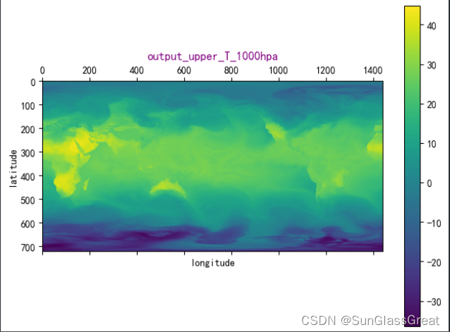
9.执行下列代码，绘制全球气温图

fig, axs = plt.subplots()
fig.tight_layout(pad=0.2, w_pad=2, h_pad=3)
cax0 = axs.matshow(output_upper[2,0]-273.15)# [2,0]:[T,1000hpa]
fig.colorbar(cax0)
axs.set_title("output_upper_T_1000hpa",loc='center',color='purple')
axs.set_xlabel("longitude")
axs.set_ylabel("latitude")


plt.show()

输出结果如下：

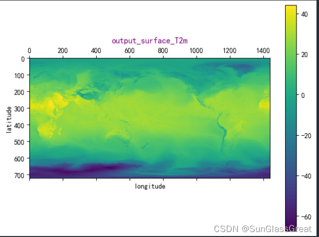
10.执行下列代码，绘制地表2m处气温图

fig, axs = plt.subplots()
fig.tight_layout(pad=0.2, w_pad=2, h_pad=3)
cax0 = axs.matshow(output_surface[3]-273.15)# [3]:[T2M]
fig.colorbar(cax0)
axs.set_title("output_surface_T2m",loc='center',color='purple')
axs.set_xlabel("longitude")
axs.set_ylabel("latitude")


plt.show()

结果如下：

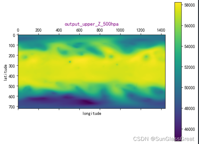
11.执行下列代码，绘制全球500hpa处的重力位势图

fig, axs = plt.subplots()
fig.tight_layout(pad=0.2, w_pad=2, h_pad=3)
cax0 = axs.matshow(output_upper[0,5])# [0,5]:[Z,500hpa]
fig.colorbar(cax0)
axs.set_title("output_upper_Z_500hpa",loc='center',color='purple')
axs.set_xlabel("longitude")
axs.set_ylabel("latitude")


plt.show()

结果如下：

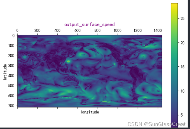
12.执行下列代码，绘制全球地表10m处风速图

fig, axs = plt.subplots()
fig.tight_layout(pad=0.2, w_pad=2, h_pad=3)
output_wspd=(output_surface[1]**2+output_surface[2]**2)**0.5
cax0 = axs.matshow(output_wspd)
fig.colorbar(cax0)
axs.set_title("output_surface_speed",loc='center',color='purple')
axs.set_xlabel("longitude")
axs.set_ylabel("latitude")


plt.show()

结果如下：