学习笔记--吴恩达 Deeplearning 第一课 第二周 逻辑回归 （答案及知识点总结）

吴恩达 深度学习 第二周 逻辑回归

程序步骤

***导入需要的函数包和给定的py文件***
import numpy as np #存储和处理大型矩阵
import matplotlib.pyplot as plt  #Python 的2D绘图库,生成绘图，直方图，功率谱，条形图，错误图，散点图等
import h5py #h5py软件包是HDF5二进制数据格式的Python接口
import scipy #处理插值、积分、优化、图像处理、常微分方程数值解的求解、信号处理等问题
from PIL import Image #python的第三方图像处理库
from scipy import ndimage #ndimage---Multi-dimensional image processing(多维图像处理包)
from lr_utils import load_dataset #老师给的文件，用来读取数据集，注意：将此文件与运行程序放到一个文件夹，以免报错
%matplotlib inline  #使能够在jupyter出图

1. 导入数据集（猫/非猫）

train_set_x_orig, train_set_y, test_set_x_orig, test_set_y, classes = load_dataset()

当我们回看lr_utils时，看到如下语句，其中读取的train_catvnoncat文件来自于老师给的datasets文件夹
train_dataset = h5py.File(‘datasets/train_catvnoncat.h5’, “r”)

文件中用到了h5py模块,关于h5py部分用法总结如下
import h5py
# 生成一个.h5文件
f = h5py.File(‘data.h5’, ‘w’)
f.create_dataset(‘X_train’, data=X) #输入
f.create_dataset(‘y_train’, data=y)。#标签
f.close()

# 导入h5文件
f = h5py.File(‘data.h5’, ‘r’)
X = f[‘X_train’]
Y = f[‘y_train’]
f.close()

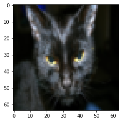
# 数据可视化
index = 25
plt.imshow(train_set_x_orig[index]) #显示了训练集输入部分第25张图片
print ("y = " + str(train_set_y[:, index]) + ", it's a '" + classes[np.squeeze(train_set_y[:, index])].decode("utf-8") +  "' picture.") #np.squeeze：从数组的形状中删除单维度条目，即把shape中为1的维度去掉

返回值：y = [1], it’s a ‘cat’ picture.

2.将三维图片展平为一维数组，实现numpy数据转换

### START CODE HERE ### (≈ 3 lines of code)
m_train = train_set_x_orig.shape[0] #训练集为四列矩阵，第一列为训练集数目，第二、三列为图片宽和高，第四列为图片的维度
m_test = test_set_x_orig.shape[0]
num_px = train_set_x_orig.shape[1]
### END CODE HERE ###

print ("Number of training examples: m_train = " + str(m_train))
print ("Number of testing examples: m_test = " + str(m_test))
print ("Height/Width of each image: num_px = " + str(num_px))
print ("Each image is of size: (" + str(num_px) + ", " + str(num_px) + ", 3)")
print ("train_set_x shape: " + str(train_set_x_orig.shape))
print ("train_set_y shape: " + str(train_set_y.shape))
print ("test_set_x shape: " + str(test_set_x_orig.shape))
print ("test_set_y shape: " + str(test_set_y.shape))

返回值：
Number of training examples: m_train = 209
Number of testing examples: m_test = 50
Height/Width of each image: num_px = 64
Each image is of size: (64, 64, 3)
train_set_x shape: (209, 64, 64, 3)
train_set_y shape: (1, 209)
test_set_x shape: (50, 64, 64, 3)
test_set_y shape: (1, 50)

接下来，我们将三维图片转化为numpy形状数组（长宽3，1），使我们的训练（和测试）数据集是一个numpy数组，其中每一列表示一个展平的图像。训练集中应有m_train训练列（测试集：m_test列）。

若矩阵x.shape = （a,b,c,d）,想将x.shape变为（bcd,a）,用下面的语句实现：
X_flatten = X.reshape(X.shape[0], -1).T

# 改变训练集和测试集的性质
### START CODE HERE ### (≈ 2 lines of code)
train_set_x_flatten = train_set_x_orig.reshape(train_set_x_orig.shape[0], -1).T
test_set_x_flatten = test_set_x_orig.reshape(test_set_x_orig.shape[0], -1).T
### END CODE HERE ###

print ("train_set_x_flatten shape: " + str(train_set_x_flatten.shape))
print ("train_set_y shape: " + str(train_set_y.shape))
print ("test_set_x_flatten shape: " + str(test_set_x_flatten.shape))
print ("test_set_y shape: " + str(test_set_y.shape))
print ("sanity check after reshaping: " + str(train_set_x_flatten[0:5,0]))

返回值：
train_set_x_flatten shape: (12288, 209)
train_set_y shape: (1, 209)
test_set_x_flatten shape: (12288, 50)
test_set_y shape: (1, 50)
sanity check after reshaping: [17 31 56 22 33]

3.数据集居中并标准化
表示彩色图像，要每个像素指定红、绿和蓝通道（RGB），因此像素值实际上是一个由0到255之间的三个数字组成的向量。
机器学习中一个常见的预处理步骤是将数据集居中并标准化，这意味着从每个示例中减去整个numpy数组的平均值，然后将每个示例除以整个numpy数组的标准差。但对于图片数据集来说，可以将数据集的每一行除以255（像素通道的最大值）。如下：

train_set_x = train_set_x_flatten/255.
test_set_x = test_set_x_flatten/255.

4.构建我们算法的部分
建立神经网络的主要步骤是：
定义模型结构（例如输入特征的数量）
初始化模型参数
循环：
计算当前损失函数（正向传播）
计算当前梯度（反向传播）
更新参数（梯度下降）
您通常分别构建1-3并将它们集成到我们称为model（）的一个函数中

# 4.1梯度函数: sigmoid

def sigmoid(z):

    ### START CODE HERE ### (≈ 1 line of code)
    s = 1/(1+np.exp(-z))
    ### END CODE HERE ###
    
    return s

print ("sigmoid([0，2]) = " + str(sigmoid(np.array([0,2]))))

返回值：sigmoid([0，2]) = [0.5 0.88079708]

# 4.2 梯度函数: 初始为0

def initialize_with_zeros(dim):
    
    ### START CODE HERE ### (≈ 1 line of code)
    w = np.zeros([dim,1])
    b = 0
    ### END CODE HERE ###

    assert(w.shape == (dim, 1))
    assert(isinstance(b, float) or isinstance(b, int))
    
    return w, b

dim = 2
w, b = initialize_with_zeros(dim)
print ("w = " + str(w))
print ("b = " + str(b))

返回值：
w = [[0.]
[0.]]
b = 0

#4.3前向传播和后向传播

def propagate(w, b, X, Y):

    m = X.shape[1]
    
    # FORWARD PROPAGATION (FROM X TO COST)
    ### START CODE HERE ### (≈ 2 lines of code)
    A = sigmoid(np.dot(w.T,X)+b)                                    # compute activation
    cost = - np.sum(Y*np.log(A)+(1-Y)*np.log(1-A))/m                              # compute cost
    ### END CODE HERE ###
    
    # BACKWARD PROPAGATION (TO FIND GRAD)
    ### START CODE HERE ### (≈ 2 lines of code)
    dw = np.dot(X,(A-Y).T)/m
    db = np.sum(A-Y)/m
    ### END CODE HERE ###

    assert(dw.shape == w.shape)
    assert(db.dtype == float)
    cost = np.squeeze(cost)
    assert(cost.shape == ())
    
    grads = {"dw": dw,
             "db": db}
    
    return grads, cost

w, b, X, Y = np.array([[1.],[2.]]), 2., np.array([[1.,2.,-1.],[3.,4.,-3.2]]), np.array([[1,0,1]])
grads, cost = propagate(w, b, X, Y)
print ("dw = " + str(grads["dw"]))
print ("db = " + str(grads["db"]))
print ("cost = " + str(cost))

返回值：
dw = [[0.99845601]
[2.39507239]]
db = 0.001455578136784208
cost = 5.801545319394553

扩展知识
np.dot()函数：对秩为1的数组，执行对应位置相乘，然后再相加；秩不为1的二维数组，执行矩阵乘法运算；
np.multiply()函数：数组和矩阵对应位置相乘，输出与相乘数组/矩阵的大小一致
星号（*）乘法运算：对数组执行对应位置相乘；对矩阵执行矩阵乘法运算
注意：累加的时候要使用np.sum，不能直接用sum,sum 不能处理二维及二维以上数组

# 4.4 最优化

def optimize(w, b, X, Y, num_iterations, learning_rate, print_cost = False):
    """
    该函数通过运行梯度下降算法优化w和b

论据：
w——权重，numpy数组大小为：（num-px*num-px*3，1）
b——偏差，标量
X——形状数据（num_px*num_px*3，样本数）
Y——形状为（1，示例数）的真“标签”向量（非猫为0，猫为1）
num_iterations——优化循环的迭代次数
learning_rate ——梯度下降更新规则的学习率
print_cost ——每100步打印一次损失

返回：
params—包含权重w和偏差b的字典
grads—包含与成本函数相关的权重和偏差梯度的字典
costs——优化过程中计算的所有成本的列表，这将用于绘制学习曲线。

提示：
你基本上需要写下两个步骤，然后重复它们：
1） 计算当前参数的成本和梯度。使用propagate（）。
2） 对w和b使用梯度下降规则更新参数。
    """
    
    costs = []
    
    for i in range(num_iterations):
        
        
        # Cost and gradient calculation (≈ 1-4 lines of code) 上一个程序框中的返回值即grads和cost
        ### START CODE HERE ### 
        grads, cost = propagate(w, b, X, Y)
        ### END CODE HERE ###
        
        # Retrieve derivatives from grads
        dw = grads["dw"]
        db = grads["db"]
        
        # update rule (≈ 2 lines of code)  由梯度下降规则可知：𝜃=𝜃−𝛼𝑑𝜃 其中𝜃是学习率（learning rate）
        ### START CODE HERE ###
        w = w - learning_rate*dw
        b = b - learning_rate*db
        ### END CODE HERE ###
        
        # Record the costs
        if i % 100 == 0:
            costs.append(cost)
        
        # Print the cost every 100 training iterations
        if print_cost and i % 100 == 0:
            print ("Cost after iteration %i: %f" %(i, cost))
    
    params = {"w": w,
              "b": b}
    
    grads = {"dw": dw,
             "db": db}
    
    return params, grads, costs

params, grads, costs = optimize(w, b, X, Y, num_iterations= 100, learning_rate = 0.009, print_cost = False)

print ("w = " + str(params["w"]))
print ("b = " + str(params["b"]))
print ("dw = " + str(grads["dw"]))
print ("db = " + str(grads["db"]))

返回值：
w = [[0.19033591]
[0.12259159]]
b = 1.9253598300845747
dw = [[0.67752042]
[1.41625495]]
db = 0.21919450454067654

# 4.5 预测

def predict(w, b, X):
    '''
    Predict whether the label is 0 or 1 using learned logistic regression parameters (w, b)
    
    Arguments:
    w -- weights, a numpy array of size (num_px * num_px * 3, 1)
    b -- bias, a scalar
    X -- data of size (num_px * num_px * 3, number of examples)
    
    Returns:
    Y_prediction -- a numpy array (vector) containing all predictions (0/1) for the examples in X
    '''
    
    m = X.shape[1]
    Y_prediction = np.zeros((1,m))
    w = w.reshape(X.shape[0], 1)
    
    # Compute vector "A" predicting the probabilities of a cat being present in the picture
    ### START CODE HERE ### (≈ 1 line of code)
    A = sigmoid(np.dot(w.T,X)+b) 
    ### END CODE HERE ###
    
    for i in range(A.shape[1]):
        
        # Convert probabilities A[0,i] to actual predictions p[0,i]
        ### START CODE HERE ### (≈ 4 lines of code)
        if A[0,i] < 0.5:
            Y_prediction[0,i] = 0
        else:
            Y_prediction[0,i] = 1
        ### END CODE HERE ###
    
    assert(Y_prediction.shape == (1, m))
    
    return Y_prediction

w = np.array([[0.1124579],[0.23106775]])
b = -0.3
X = np.array([[1.,-1.1,-3.2],[1.2,2.,0.1]])
print ("predictions = " + str(predict(w, b, X)))

返回值：
predictions = [[1. 1. 0.]]

5.将所有函数合并到模型中

# GRADED FUNCTION: model

def model(X_train, Y_train, X_test, Y_test, num_iterations = 2000, learning_rate = 0.5, print_cost = False):
    """
   通过调用前面实现的函数来构建逻辑回归模型

论据：
X_train——由numpy形状数组表示的训练集（num_px*num_px*3，m_train）
Y_train—由形状为（1，m_train）的numpy数组（向量）表示的训练标签
X_test——由一个numpy形状数组表示的测试集（num_px*num_px*3，m_test）
Y_检验——由形状为（1，m_test）的numpy数组（向量）表示的检验标签
num_iterations——表示优化参数的迭代次数的超参数
learning_rate——表示optimize（）更新规则中使用的学习率的超参数
print_cost—设置为true以每100次迭代打印一次成本

返回：
d——包含模型信息的字典。
    """
    
    ### START CODE HERE ###
    
    # initialize parameters with zeros (≈ 1 line of code)
    w, b = initialize_with_zeros(X_train.shape[0])

    # Gradient descent (≈ 1 line of code)
    parameters, grads, costs = optimize(w, b, X_train, Y_train, num_iterations, learning_rate, print_cost = False)
    
    # Retrieve parameters w and b from dictionary "parameters"
    w = parameters["w"]
    b = parameters["b"]
    
    # Predict test/train set examples (≈ 2 lines of code)
    Y_prediction_test = predict(w, b, X_test)
    Y_prediction_train = predict(w, b, X_train)

    ### END CODE HERE ###

    # Print train/test Errors
    print("train accuracy: {} %".format(100 - np.mean(np.abs(Y_prediction_train - Y_train)) * 100))
    print("test accuracy: {} %".format(100 - np.mean(np.abs(Y_prediction_test - Y_test)) * 100))

    
    d = {"costs": costs,
         "Y_prediction_test": Y_prediction_test, 
         "Y_prediction_train" : Y_prediction_train, 
         "w" : w, 
         "b" : b,
         "learning_rate" : learning_rate,
         "num_iterations": num_iterations}
    
    return d

d = model( train_set_x,train_set_y, test_set_x, test_set_y, num_iterations = 2000, learning_rate = 0.005, print_cost = True)

返回值：
train accuracy: 99.04306220095694 %
test accuracy: 70.0 %

点评：训练准确率接近100%。这是一个很好的健全性检查：您的模型正在工作，并且具有足够高的容量来适应培训数据。测试误差为72%。考虑到我们使用的数据集很小，而且logistic回归是一个线性分类器，所以对于这个简单的模型来说，这并不坏。但不用担心，下周你会建立一个更好的分类器！
此外，您还可以看到，该模型显然过度拟合了训练数据。之后，您将学习如何减少过度拟合，例如使用正则化。使用下面的代码（并更改索引变量），您可以查看测试集图片上的预测。

# 被错误分类的图片示例
index = 1
plt.imshow(test_set_x[:,index].reshape((num_px, num_px, 3)))
print ("y = " + str(test_set_y[0,index]) + ", you predicted that it is a \"" + classes[int(d["Y_prediction_test"][0,index])].decode("utf-8") +  "\" picture.")

注意：此处会报错，需要将d[“Y_prediction_test”][0,index]转化为整型

# 显示训练过程中costs的变化曲线
costs = np.squeeze(d['costs'])
plt.plot(costs)
plt.ylabel('cost')
plt.xlabel('iterations (per hundreds)')
plt.title("Learning rate =" + str(d["learning_rate"]))
plt.show()

解读：你可以看到costs在下降。这表明参数正在学习中。但是，你可以看到你可以在训练集上训练更多的次数。尝试增加上面单元格中的迭代次数并重新运行单元格。你可能会看到训练集的准确性上升，但测试集的准确性下降。这被称为过度拟合。

6.进一步分析（可选/非分级练习）
学习率的选择
提醒：为了使梯度下降起作用，你必须明智地选择学习率。学习率α确定更新参数的速度。如果学习率太大，我们可能会“超调”最佳值。同样，如果它太小，我们将需要太多的迭代来收敛到最佳值。这就是为什么使用调整好的学习率是至关重要的。
让我们将模型的学习曲线与几种学习率的选择进行比较。运行下面的单元格。这大概需要1分钟。也可以尝试不同于我们初始化的learning_rates变量所包含的三个值的值，然后看看会发生什么。

learning_rates = [0.01, 0.001, 0.0001]
models = {}
for i in learning_rates:
    print ("learning rate is: " + str(i))
    models[str(i)] = model(train_set_x, train_set_y, test_set_x, test_set_y, num_iterations = 1500, learning_rate = i, print_cost = False)
    print ('\n' + "-------------------------------------------------------" + '\n')

for i in learning_rates:
    plt.plot(np.squeeze(models[str(i)]["costs"]), label= str(models[str(i)]["learning_rate"]))

plt.ylabel('cost')
plt.xlabel('iterations (hundreds)')

legend = plt.legend(loc='upper center', shadow=True)
frame = legend.get_frame()
frame.set_facecolor('0.90')
plt.show()

返回值：
learning rate is: 0.01
train accuracy: 99.52153110047847 %
test accuracy: 68.0 %

---

learning rate is: 0.001
train accuracy: 88.99521531100478 %
test accuracy: 64.0 %

---

learning rate is: 0.0001
train accuracy: 68.42105263157895 %
test accuracy: 36.0 %

---

解释：
不同的学习率会产生不同的costs，从而产生不同的预测结果。
如果学习率太大（0.01），成本函数可能上下波动。它甚至可能会发散（尽管本例中，使用0.01最终还是会得到很好的成本值）。
低costs并不意味着更好的模式。你得检查一下是否有过度拟合的可能。当训练精度远高于测试精度时就会发生这种情况。
在深入学习中，我们通常建议您：
选择学习率，更好地最小化成本函数。如您的模型过拟合，请用其他技术来减少过拟合。

7.用自己的图片进行验证
祝贺你完成这项任务。您可以使用自己的图像并查看模型的输出。要做到这一点：
1.点击本笔记本上栏的“文件”，然后点击“打开”进入Coursera Hub。
2.将图像添加到此Jupyter笔记本的“image s”文件夹中
3.在下面的代码中更改图像的名称
4.运行代码并检查算法是否正确（1=cat，0=非cat）！

import imageio
from skimage.transform import resize
## START CODE HERE ## (PUT YOUR IMAGE NAME) 
my_image = "dog.jpeg"   # change this to the name of your image file 
## END CODE HERE ##

# We preprocess the image to fit your algorithm.
fname = "images/" + my_image
~~#image = np.array(ndimage.imread(fname, flatten=False))~~ 
image = np.array(imageio.imread(fname))
~~#my_image = scipy.misc.imresize(image, size=(num_px,num_px)).reshape((1, num_px*num_px*3)).T~~ 
my_image = resize(image, output_shape=(num_px,num_px)).reshape((1, num_px*num_px*3)).T
my_predicted_image = predict(d["w"], d["b"], my_image)

plt.imshow(image)
print("y = " + str(np.squeeze(my_predicted_image)) + ", your algorithm predicts a \"" + classes[int(np.squeeze(my_predicted_image)),].decode("utf-8") +  "\" picture.")

返回值：
y = 0.0, your algorithm predicts a “non-cat” picture.

注意：运行原始代码时，我这边会报错“module ‘scipy.misc’ has no attribute ‘imread’”和“module ‘scipy.misc’ has no attribute ‘imresize’”，所以我把程序改了下，就可以成功运行了。记得把自己的图片放到image文件夹中哦！