Machine_Learning_Regularization

In this chapter, we introduce regularization methods with some hands-on Python codes~

Regularization

• Why regularization: in the bias-variance trade-off, we have shown that some complicated models will have quite low bias, however they will get overfitted because the model contains a lot of bias – which means that their model has captured some noise in their training set. So we need to control the variance.
• How regularization: Through constraining or regularizing the coefficient estimates, or equivalently, shrinking the coefficient estimates toward zero, we can reduce the variance of the model.

Lasso

The idea of lasso is to use $l1$ penalty that has the effect of the forcing some of the coefficient estimats to be exactly equal to 0 when the tuning parameter $\alpha$ is sufficiently large. This is called sparse solutions of linear models penalized with the $l1$ norm.

• Mathematically, it consists of a linear model with an added regularization term or shrinkage penalty.
  
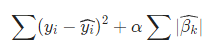
  Here we can see that, all the $\beta$'s are penalized equally.
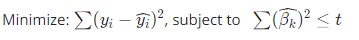
  An equivalent optimization problem:
  
• $\alpha$ is called a tuning parameter. When $\alpha$ is greater, the coefficient estimation will be smaller.
• Lasso is able to do variable selection. And it is simpler and more interpretable.

from sklearn import linear_model
reg=linear_model.Lasso(alpha=0.1)
reg.fit([[0,0],[1,1]],[0,1])
reg.predict([[1,1]])

Ridge

The idea of ridge is just like Lass - we add an regularization term. However, this time we use $l2$ norm.

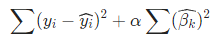
or the same opt problem:

• Why $l2$ norm: $l2$ norm will penalize greater $\beta$'s more heavily.
• Cannot do variable selection
• Ridge’s solution is close to linear regression: $\beta =(X^{T}X+\alpha I{)}^{-1}{X}^{T}Y$
• Ridge is quite quickly because for a fixed α, we only need to estimate 1 single model. Instead, ols will need to find $2^n$ of stepwise models.
  
  
  In some cases we may get more features than variables, typically in healthcare data.
• If we have $n$ obs and $k$ variables and $k>n$, using Lasso will produce only $n$ variables, but ridge will still remain all $k$ variables because Lasso does not have a solution in this case (no $X^{-1}$)
• For this dataset, if we only use linear regression, we will not be able to estimate a model neither. But in ridge, we could still get a model because we can get $(X^{T}X+\alpha I{)}^{-1}$
  
  

Elastic Net

Elastic-net is a weighted combination of Ridge and Lasso:

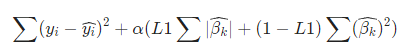
or equivalent opt problem

Especially, Elastic-Net reduces to Lasso when L=1, while reduces to Ridge when L=0.

• Why elasic net and lasso can do variable selection but ridge cannot: Lasso and Elastic Net regression have corners. As a result, we might have a $\hat{\beta }$ value being 0. However, since Ridge does not have corners, we will not be able to get a $\hat{\beta }$ value being 0. Thus, Lasso and Elastic net can both be used for variable selection, while Ridge cannot.
• Comparing Lasso and Elastic Net, Lasso has sharper corners. Thus, it will more aggressively reduce the number of variables comparing to Elastic Net. Elastic Net, on the other hand, is more gentle with variable selection.

• In this picture, The ellipse is the contour of RSS.
• Ridge regression has a circular constraint with no sharp points, while Lasso and Elastic Net both have corners on the axis. The intersection of Ridge RSS will not generally occur on an axis, so its coeffeicient estimates will be exclusively non-zero.

Lasso: a real case

In lasso, we care about the parameter $\alpha$. We will use cross validation to find it.

GridSearchCV

from sklearn import datasets
X, y = datasets.load_diabetes(return_X_y=True)

lasso = Lasso()

cv = RepeatedKFold(n_splits=10, n_repeats=3, random_state=1)

lasso_alphas = np.linspace(0.01, 0.1, 20)
grid = dict()
grid['alpha'] = lasso_alphas
gscv = GridSearchCV(lasso, grid, cv = cv, n_jobs=-1)

results = gscv.fit(X, y)

print('MSE:  %.5f ' % results.best_score_)
print('Config: %s ' % results.best_params_)
plt.plot(lasso_alphas, results.cv_results_['mean_test_score'])
plt.xlim(0.01, 0.1)
plt.show()

MSE:  0.47184 
Config: {'alpha': 0.019473684210526317}

LassoCV

Spcifically for lasso. sklearn_linear_model.LassoCV

LassoCV(eps, n_alphas=100, alphas=ndarray, fit_intercept = True, normalize=False, cv=int, random_state=, n_jobs)

• n_jobs: Number of CPUs to use during the cross validation
• .score(X, y): Return the coefficient of determination of the prediction.
• .alpha_ Best alpha
• .mse_path_ All mse’s wrt each alpha
• .alphas_
• .coef_ Coefficients for each variable

from sklearn.linear_model import LassoCV
lassocv = LassoCV(cv=20, random_state=0).fit(X, y)

print('Score: %.5f' % lassocv.score(X, y))
print(lassocv.predict(X[:1,]))
print('Alpha: %.5f' % lassocv.alpha_)
print(lassocv.coef_)

Score: 0.53886
[197.0943]
Alpha: 0.03265
[  -0.     -217.6243  525.7042  299.8325 -112.4265   -0.     -244.4867
    0.      497.7109   87.9674  -15.3141  -42.8252   34.8853  -63.6733
  -52.1601   50.1955   30.108   -63.8399  -30.2097   72.6927   61.6619
   47.4095  119.0708   41.8884]

Plot the mse path:

# Author: Olivier Grisel, Gael Varoquaux, Alexandre Gramfort
# License: BSD 3 clause
# #############################################################################
# LassoCV: coordinate descent

# Compute paths
print("Computing regularization path using the coordinate descent lasso...")
t1 = time.time()
model = LassoCV(cv=20).fit(X, y)
t_lasso_cv = time.time() - t1

# Display results
plt.figure()
ymin, ymax = 2300, 3800
plt.semilogx(model.alphas_ + EPSILON, model.mse_path_, ':')
plt.plot(model.alphas_ + EPSILON, model.mse_path_.mean(axis=-1), 'k',
         label='Average across the folds', linewidth=2)
plt.axvline(model.alpha_ + EPSILON, linestyle='--', color='k',
            label='alpha: CV estimate ' + str(round(model.alpha_, 3)))

plt.legend()

plt.xlabel(r'$\alpha$')
plt.ylabel('Mean square error')
plt.title('Mean square error on each fold: coordinate descent '
          '(train time: %.2fs)' % t_lasso_cv)
plt.axis('tight')
plt.ylim(ymin, ymax)

# #############################################################################
# LassoLarsCV: least angle regression

# Compute paths
print("Computing regularization path using the Lars lasso...")
t1 = time.time()
model = LassoLarsCV(cv=20, normalize=False).fit(X, y)
t_lasso_lars_cv = time.time() - t1

# Display results
plt.figure()
plt.semilogx(model.cv_alphas_ + EPSILON, model.mse_path_, ':')
plt.semilogx(model.cv_alphas_ + EPSILON, model.mse_path_.mean(axis=-1), 'k',
             label='Average across the folds', linewidth=2)
plt.axvline(model.alpha_, linestyle='--', color='k',
            label='alpha CV ' + str(round(model.alpha_, 3)))
plt.legend()

plt.xlabel(r'$\alpha$')
plt.ylabel('Mean square error')
plt.title('Mean square error on each fold: Lars (train time: %.2fs)'
          % t_lasso_lars_cv)
plt.axis('tight')
plt.ylim(ymin, ymax)

plt.show()

LassoLarsIC

I edited the code to show the aic and bic value.

# Author: Olivier Grisel, Gael Varoquaux, Alexandre Gramfort
# License: BSD 3 clause

import time

import numpy as np
import matplotlib.pyplot as plt

from sklearn.linear_model import LassoCV, LassoLarsCV, LassoLarsIC
from sklearn import datasets

# This is to avoid division by zero while doing np.log10
EPSILON = 1e-4

X, y = datasets.load_diabetes(return_X_y=True)

rng = np.random.RandomState(42)
X = np.c_[X, rng.randn(X.shape[0], 14)]  # add some bad features

# normalize data as done by Lars to allow for comparison
X /= np.sqrt(np.sum(X ** 2, axis=0))

# #############################################################################
# LassoLarsIC: least angle regression with BIC/AIC criterion

model_bic = LassoLarsIC(criterion='bic', normalize=False)
t1 = time.time()
model_bic.fit(X, y)
t_bic = time.time() - t1
alpha_bic_ = model_bic.alpha_

model_aic = LassoLarsIC(criterion='aic', normalize=False)
model_aic.fit(X, y)
alpha_aic_ = model_aic.alpha_


def plot_ic_criterion(model, name, color, ic):
    criterion_ = model.criterion_
    plt.semilogx(model.alphas_ + EPSILON, criterion_, '--', color=color,
                 linewidth=3, label='%s criterion' % name)
    vertical_label = 'alpha: %s estimate ' % name
    vertical_label += str(round(ic, 3))
    plt.axvline(model.alpha_ + EPSILON, color=color, linewidth=3,
                label= vertical_label )
    plt.xlabel(r'$\alpha$')
    plt.ylabel('criterion')


plt.figure()
plot_ic_criterion(model_aic, 'AIC', 'b', alpha_aic_)
plot_ic_criterion(model_bic, 'BIC', 'r', alpha_bic_)
plt.legend()
plt.title('Information-criterion for model selection (training time %.3fs)'
          % t_bic)
plt.show()

Source:

Business Analytics - Yi Zhang
ISLR
sklearn