


本博客来源于CSDN机器鱼,未同意任何人转载。
更多内容,欢迎点击本专栏目录,查看更多内容。
目录
0 引言
基于MATLAB2020b的深度学习框架,提出了一种基于CNN-LSTM的多变量电力负荷预测方法,该方法将历史负荷与气象的多变量时间序列数据作为输入,以当天的96个时刻负荷值为输出,建模学习特征内部动态变化规律,即多变量输入多输出模型。同时,针对该模型超参数选择困难的问题,提出利用人工大猩猩部队GTO算法实现该模型超参数的优化选择。
1 数据准备
数据为2016电工杯的电力负荷数据,数据可以在【这里】下载得到。数据包含20140101到20250110的375天多变量数据。每天含96个时刻的负荷数据,即每间隔15分钟采集一次;以及当天的最高温度℃、最低温度℃、平均温度℃、相对湿度(平均)、降雨量(mm),即一天101个数据。
我们做时间序列预测,采用的是滚动序列建模,即采用1到n天的n*101个值为输入,第n+1天的96个负荷做输出,然后第2到n+1天的n*101个值为输入,第n+2天的96个负荷值为输出,这样进行滚动序列建模。数据划分的代码如下,我先区分了负荷数据与气象数据,然后分别归一化再划分数据集,其实应该先划分数据,再对训练集归一化,然后用训练集的参数对测试集(验证集)做归一化,这个就不要纠结了,想改的自己改一下:
clc;clear;close all;
%%
data=xlsread('电荷数据.csv','B2:CX376');
%负荷数据--每天96个负荷值,气象数据 最高温度℃	最低温度℃ 平均温度℃ 相对湿度(平均) 降雨量(mm)
power=data(:,1:96);
weather=data(:,97:end);
% 归一化 或者 标准化 看哪个效果好
method=@mapminmax;%  mapstd mapminmax
[x1,mappingx1]=method(power');
[x2,mappingx2]=method(weather');
data=[x1' x2'];
% 前steps天steps*101 为输入,来预测未来一天的96负荷值 为输出
steps=10;
samples=size(data,1)-steps;%样本数
for i=1:samples
    input{i,:}=data(i:i+steps-1,:);
    output(i,:)=data(i+steps,1:96);
end
%% 数据划分 8:1:1划分训练集、验证集、测试集
n_samples=size(input,1);
n=1:n_samples;%顺序划分用这个n
m1=round(0.8*n_samples);
m2=round(0.9*n_samples);

Train_X=input(n(1:m1));
Train_Y=output(n(1:m1),:);

Val_X=input(n(m1+1:m2));
Val_Y=output(n(m1+1:m2),:);

Ttest_X=input(n(m2+1:end));
Ttest_Y=output(n(m2+1:end),:);
2 CNN-LSTM模型搭建
MATLAB2020b自带的深度学习框架,其中会用到convolution2dLayer,sequenceFoldingLayer,reluLayer,averagePooling2dLayer,lstmLayer,fullyConnectedLayer等。需要的函数主要参考【这里】,据此我们建立CNN-LSTM模型如下:
clc;clear;close all;
%%
data=xlsread('电荷数据.csv','B2:CX376');
%负荷数据--每天96各负荷值,气象数据 最高温度℃ 最低温度℃ 平均温度℃ 相对湿度(平均) 降雨量(mm)
power=data(:,1:96);
weather=data(:,97:end);
% 归一化 或者 标准化 看哪个效果好
method=@mapminmax;% mapstd mapminmax
[x1,mappingx1]=method(power');
[x2,mappingx2]=method(weather');
data=[x1' x2'];
% 前steps天steps*101 为输入,来预测未来一天的96负荷值 为输出
steps=10;
samples=size(data,1)-steps;%样本数
for i=1:samples
input{i,:}=data(i:i+steps-1,:);
output(i,:)=data(i+steps,1:96);
end
%% 数据划分 8:1:1划分训练集、验证集、测试集
n_samples=size(input,1);
n=1:n_samples;%顺序划分用这个n
m1=round(0.8*n_samples);
m2=round(0.9*n_samples);
Train_X=input(n(1:m1));
Train_Y=output(n(1:m1),:);
Val_X=input(n(m1+1:m2));
Val_Y=output(n(m1+1:m2),:);
Ttest_X=input(n(m2+1:end));
Ttest_Y=output(n(m2+1:end),:);
%% 网络搭建
lr=0.001;
epochs=100;
miniBatchSize = 32;
kernel1_num=8;
kernel1_size=3;
pool1_size=2;
kernel2_num=16;
kernel2_size=3;
pool2_size=2;
lstm_node=20;
fc_node=100;
rng(0)
input_size=[size(Train_X{1}) 1];
output_size=size(Train_Y,2);
layers = [
sequenceInputLayer(input_size,"Name","sequence")
sequenceFoldingLayer("Name","seqfold")
convolution2dLayer([kernel1_size kernel1_size],kernel1_num,"Name","conv_1","Padding","same")
reluLayer("Name","relu_1")
averagePooling2dLayer([1 pool1_size],"Name","avgpool2d_1")
convolution2dLayer([kernel2_size kernel2_size],kernel2_num,"Name","conv_2","Padding","same")
reluLayer("Name","relu_2")
averagePooling2dLayer([1 pool2_size],"Name","avgpool2d_2")
sequenceUnfoldingLayer("Name","sequnfold")
flattenLayer("Name","flatten")
lstmLayer(lstm_node,"Name","lstm",'OutputMode','last')
fullyConnectedLayer(fc_node,"Name","fc")
reluLayer("Name","relu_3")
fullyConnectedLayer(output_size,"Name","out")
regressionLayer("Name","regressionoutput")];
lgraph = layerGraph(layers);
lgraph = connectLayers(lgraph,"seqfold/miniBatchSize","sequnfold/miniBatchSize");
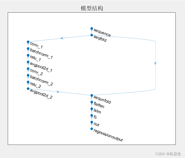
figure
plot(lgraph)
title("模型结构")
options = trainingOptions('adam', ...
'MiniBatchSize',miniBatchSize, ...
'MaxEpochs',epochs, ...
'InitialLearnRate',lr,...
'LearnRateSchedule','piecewise',...
'LearnRateDropFactor',1,...
'Shuffle','every-epoch', ...
'ValidationData',{Val_X,Val_Y}, ...
'Verbose',1);
train_again=1;% 为1就代码重新训练模型,为0就是调用训练好的网络
if train_again==1
[net,traininfo] = trainNetwork(Train_X,Train_Y,lgraph,options);
save result/cnn_lstm_net net traininfo
else
load result/cnn_lstm_net
end
figure
plot(traininfo.TrainingLoss);
grid on
title('CNN-LSTM');
xlabel('训练次数');
ylabel('损失值');
%% 预测,
YPred1=predict(net,Ttest_X);
YPred1=method('reverse',YPred1',mappingx1);
Ytest1=method('reverse',Ttest_Y',mappingx1);
[m,n]=size(Ytest1);
real=reshape(Ytest1,[1,m*n]);
pred=reshape(YPred1,[1,m*n]);
result(real,pred,'CNN-LSTM')
save result/cnn_lstm_result real pred
figure
plot(real)
hold on;grid on
plot(pred)
legend('真实值','预测值')function result(true_value,predict_value,type)
disp(type)
rmse=sqrt(mean((true_value-predict_value).^2));
disp(['根均方差(RMSE):',num2str(rmse)])
mae=mean(abs(true_value-predict_value));
disp(['平均绝对误差(MAE):',num2str(mae)])
mape=mean(abs((true_value-predict_value)./true_value));
disp(['平均相对百分误差(MAPE):',num2str(mape*100),'%'])
R2 = 1 - norm(true_value-predict_value)^2/norm(true_value - mean(true_value))^2;
disp(['决定系数(R2):',num2str(R2)])
fprintf('\n')我们输入的是[batchsize steps 101],MATLAB的这个convolution2dLayer是2d卷积,不符合我们输入结构,好在提供了sequenceInputLayer,sequenceFoldingLayer,sequenceUnfoldingLayer这几个函数,专门用来接收这样的数据以便于连接conv2d与lstm。
与此同时,观察模型搭建那里,我们发现有很多参数需要进行手动设置,这个参数直接影响最后的结果,而设置这些参数我们是没有指导方法的,因此需要采用某些智能算法来优化选择。
lr=0.001;
epochs=100;
miniBatchSize = 32;
kernel1_num=8;
kernel1_size=3;
pool1_size=2;
kernel2_num=16;
kernel2_size=3;
pool2_size=2;
lstm_node=20;
fc_node=100;
3 GTO超参数优化
3.1 GTO函数极值寻优
首先贴一下网上找的GTO函数极值寻优代码,如下:
function [Silverback_Score,Silverback,convergence_curve]=GTO(pop_size,max_iter,lower_bound,upper_bound,variables_no,fobj)


% initialize Silverback
Silverback=[];
Silverback_Score=inf;

%Initialize the first random population of Gorilla
X=initialization(pop_size,variables_no,upper_bound,lower_bound);


convergence_curve=zeros(max_iter,1);

for i=1:pop_size
    Pop_Fit(i)=fobj(X(i,:));%#ok
    if Pop_Fit(i)<Silverback_Score
        Silverback_Score=Pop_Fit(i);
        Silverback=X(i,:);
    end
end


GX=X(:,:);
lb=ones(1,variables_no).*lower_bound;
ub=ones(1,variables_no).*upper_bound;

%%  Controlling parameter

p=0.03;
Beta=3;
w=0.8;

%%Main loop
for It=1:max_iter

    a=(cos(2*rand)+1)*(1-It/max_iter);
    C=a*(2*rand-1);

    %% Exploration:

    for i=1:pop_size
        if rand<p
            GX(i,:) =(ub-lb)*rand+lb;
        else
            if rand>=0.5
                Z = unifrnd(-a,a,1,variables_no);
                H=Z.*X(i,:);
                GX(i,:)=(rand-a)*X(randi([1,pop_size]),:)+C.*H;
            else
                GX(i,:)=X(i,:)-C.*(C*(X(i,:)- GX(randi([1,pop_size]),:))+rand*(X(i,:)-GX(randi([1,pop_size]),:))); %ok ok

            end
        end
    end

    GX = boundaryCheck(GX, lower_bound, upper_bound);

    % Group formation operation
    for i=1:pop_size
        New_Fit= fobj(GX(i,:));
        if New_Fit<Pop_Fit(i)
            Pop_Fit(i)=New_Fit;
            X(i,:)=GX(i,:);
        end
        if New_Fit<Silverback_Score
            Silverback_Score=New_Fit;
            Silverback=GX(i,:);
        end
    end

    %% Exploitation:
    for i=1:pop_size
        if a>=w
            g=2^C;
            delta= (abs(mean(GX)).^g).^(1/g);
            GX(i,:)=C*delta.*(X(i,:)-Silverback)+X(i,:);
        else

            if rand>=0.5
                h=randn(1,variables_no);
            else
                h=randn(1,1);
            end
            r1=rand;
            GX(i,:)= Silverback-(Silverback*(2*r1-1)-X(i,:)*(2*r1-1)).*(Beta*h);

        end
    end

    GX = boundaryCheck(GX, lower_bound, upper_bound);

    % Group formation operation
    for i=1:pop_size
        New_Fit= fobj(GX(i,:));
        if New_Fit<Pop_Fit(i)
            Pop_Fit(i)=New_Fit;
            X(i,:)=GX(i,:);
        end
        if New_Fit<Silverback_Score
            Silverback_Score=New_Fit;
            Silverback=GX(i,:);
        end
    end

    convergence_curve(It)=Silverback_Score;

end
end

% This function initialize the first population of search agents
function Positions=initialization(SearchAgents_no,dim,ub,lb)

Boundary_no= size(ub,2); % numnber of boundaries

% If the boundaries of all variables are equal and user enter a signle
% number for both ub and lb
if Boundary_no==1
    Positions=rand(SearchAgents_no,dim).*(ub-lb)+lb;
end

% If each variable has a different lb and ub
if Boundary_no>1
    for i=1:dim
        ub_i=ub(i);
        lb_i=lb(i);
        Positions(:,i)=rand(SearchAgents_no,1).*(ub_i-lb_i)+lb_i;
    end
end
end
function [ X ] = boundaryCheck(X, lb, ub)

for i=1:size(X,1)
    FU=X(i,:)>ub;
    FL=X(i,:)<lb;
    X(i,:)=(X(i,:).*(~(FU+FL)))+ub.*FU+lb.*FL;
end
end
% This function draw the benchmark functions
function func_plot(func_name)
[lb,ub,dim,fobj]=Get_Functions_details(func_name);
switch func_name
case 'F1'
x=-100:2:100; y=x; %[-100,100]
case 'F2'
x=-100:2:100; y=x; %[-10,10]
case 'F3'
x=-100:2:100; y=x; %[-100,100]
case 'F4'
x=-100:2:100; y=x; %[-100,100]
case 'F5'
x=-200:2:200; y=x; %[-5,5]
case 'F6'
x=-100:2:100; y=x; %[-100,100]
case 'F7'
x=-1:0.03:1; y=x %[-1,1]
case 'F8'
x=-500:10:500;y=x; %[-500,500]
case 'F9'
x=-5:0.1:5; y=x; %[-5,5]
case 'F10'
x=-20:0.5:20; y=x;%[-500,500]
case 'F11'
x=-500:10:500; y=x;%[-0.5,0.5]
case 'F12'
x=-10:0.1:10; y=x;%[-pi,pi]
case 'F13'
x=-5:0.08:5; y=x;%[-3,1]
case 'F14'
x=-100:2:100; y=x;%[-100,100]
case 'F15'
x=-5:0.1:5; y=x;%[-5,5]
case 'F16'
x=-1:0.01:1; y=x;%[-5,5]
case 'F17'
x=-5:0.1:5; y=x;%[-5,5]
case 'F18'
x=-5:0.06:5; y=x;%[-5,5]
case 'F19'
x=-5:0.1:5; y=x;%[-5,5]
case 'F20'
x=-5:0.1:5; y=x;%[-5,5]
case 'F21'
x=-5:0.1:5; y=x;%[-5,5]
case 'F22'
x=-5:0.1:5; y=x;%[-5,5]
case 'F23'
x=-5:0.1:5; y=x;%[-5,5]
end
L=length(x);
f=[];
for i=1:L
for j=1:L
if strcmp(func_name,'F15')==0 && strcmp(func_name,'F19')==0 && strcmp(func_name,'F20')==0 && strcmp(func_name,'F21')==0 && strcmp(func_name,'F22')==0 && strcmp(func_name,'F23')==0
f(i,j)=fobj([x(i),y(j)]);
end
if strcmp(func_name,'F15')==1
f(i,j)=fobj([x(i),y(j),0,0]);
end
if strcmp(func_name,'F19')==1
f(i,j)=fobj([x(i),y(j),0]);
end
if strcmp(func_name,'F20')==1
f(i,j)=fobj([x(i),y(j),0,0,0,0]);
end
if strcmp(func_name,'F21')==1 || strcmp(func_name,'F22')==1 ||strcmp(func_name,'F23')==1
f(i,j)=fobj([x(i),y(j),0,0]);
end
end
end
surfc(x,y,f,'LineStyle','none');
end
% This function containts full information and implementations of the benchmark
% lb is the lower bound: lb=[lb_1,lb_2,...,lb_d]
% up is the uppper bound: ub=[ub_1,ub_2,...,ub_d]
% dim is the number of variables (dimension of the problem)

function [lb,ub,dim,fobj] = Get_Functions_details(F)


switch F
    case 'F1'
        fobj = @F1;
        lb=-100;
        ub=100;
        dim=30;

    case 'F2'
        fobj = @F2;
        lb=-10;
        ub=10;
        dim=30;

    case 'F3'
        fobj = @F3;
        lb=-100;
        ub=100;
        dim=30;

    case 'F4'
        fobj = @F4;
        lb=-100;
        ub=100;
        dim=30;

    case 'F5'
        fobj = @F5;
        lb=-30;
        ub=30;
        dim=30;

    case 'F6'
        fobj = @F6;
        lb=-100;
        ub=100;
        dim=30;

    case 'F7'
        fobj = @F7;
        lb=-1.28;
        ub=1.28;
        dim=30;

    case 'F8'
        fobj = @F8;
        lb=-500;
        ub=500;
        dim=30;

    case 'F9'
        fobj = @F9;
        lb=-5.12;
        ub=5.12;
        dim=30;

    case 'F10'
        fobj = @F10;
        lb=-32;
        ub=32;
        dim=30;

    case 'F11'
        fobj = @F11;
        lb=-600;
        ub=600;
        dim=30;

    case 'F12'
        fobj = @F12;
        lb=-50;
        ub=50;
        dim=30;

    case 'F13'
        fobj = @F13;
        lb=-50;
        ub=50;
        dim=30;

    case 'F14'
        fobj = @F14;
        lb=-65.536;
        ub=65.536;
        dim=2;

    case 'F15'
        fobj = @F15;
        lb=-5;
        ub=5;
        dim=4;

    case 'F16'
        fobj = @F16;
        lb=-5;
        ub=5;
        dim=2;

    case 'F17'
        fobj = @F17;
        lb=[-5,0];
        ub=[10,15];
        dim=2;

    case 'F18'
        fobj = @F18;
        lb=-2;
        ub=2;
        dim=2;

    case 'F19'
        fobj = @F19;
        lb=0;
        ub=1;
        dim=3;

    case 'F20'
        fobj = @F20;
        lb=0;
        ub=1;
        dim=6;

    case 'F21'
        fobj = @F21;
        lb=0;
        ub=10;
        dim=4;

    case 'F22'
        fobj = @F22;
        lb=0;
        ub=10;
        dim=4;

    case 'F23'
        fobj = @F23;
        lb=0;
        ub=10;
        dim=4;
end

end

% F1

function o = F1(x)
o=sum(x.^2);
end

% F2

function o = F2(x)
o=sum(abs(x))+prod(abs(x));
end

% F3

function o = F3(x)
dim=size(x,2);
o=0;
for i=1:dim
    o=o+sum(x(1:i))^2;
end
end

% F4

function o = F4(x)
o=max(abs(x));
end

% F5

function o = F5(x)
dim=size(x,2);
o=sum(100*(x(2:dim)-(x(1:dim-1).^2)).^2+(x(1:dim-1)-1).^2);
end

% F6

function o = F6(x)
o=sum(abs((x+.5)).^2);
end

% F7

function o = F7(x)
dim=size(x,2);
o=sum([1:dim].*(x.^4))+rand;
end

% F8

function o = F8(x)
o=sum(-x.*sin(sqrt(abs(x))));
end

% F9

function o = F9(x)
dim=size(x,2);
o=sum(x.^2-10*cos(2*pi.*x))+10*dim;
end

% F10

function o = F10(x)
dim=size(x,2);
o=-20*exp(-.2*sqrt(sum(x.^2)/dim))-exp(sum(cos(2*pi.*x))/dim)+20+exp(1);
end

% F11

function o = F11(x)
dim=size(x,2);
o=sum(x.^2)/4000-prod(cos(x./sqrt([1:dim])))+1;
end

% F12

function o = F12(x)
dim=size(x,2);
o=(pi/dim)*(10*((sin(pi*(1+(x(1)+1)/4)))^2)+sum((((x(1:dim-1)+1)./4).^2).*...
(1+10.*((sin(pi.*(1+(x(2:dim)+1)./4)))).^2))+((x(dim)+1)/4)^2)+sum(Ufun(x,10,100,4));
end

% F13

function o = F13(x)
dim=size(x,2);
o=.1*((sin(3*pi*x(1)))^2+sum((x(1:dim-1)-1).^2.*(1+(sin(3.*pi.*x(2:dim))).^2))+...
((x(dim)-1)^2)*(1+(sin(2*pi*x(dim)))^2))+sum(Ufun(x,5,100,4));
end

% F14

function o = F14(x)
aS=[-32 -16 0 16 32 -32 -16 0 16 32 -32 -16 0 16 32 -32 -16 0 16 32 -32 -16 0 16 32;,...
-32 -32 -32 -32 -32 -16 -16 -16 -16 -16 0 0 0 0 0 16 16 16 16 16 32 32 32 32 32];

for j=1:25
    bS(j)=sum((x'-aS(:,j)).^6);
end
o=(1/500+sum(1./([1:25]+bS))).^(-1);
end

% F15

function o = F15(x)
aK=[.1957 .1947 .1735 .16 .0844 .0627 .0456 .0342 .0323 .0235 .0246];
bK=[.25 .5 1 2 4 6 8 10 12 14 16];bK=1./bK;
o=sum((aK-((x(1).*(bK.^2+x(2).*bK))./(bK.^2+x(3).*bK+x(4)))).^2);
end

% F16

function o = F16(x)
o=4*(x(1)^2)-2.1*(x(1)^4)+(x(1)^6)/3+x(1)*x(2)-4*(x(2)^2)+4*(x(2)^4);
end

% F17

function o = F17(x)
o=(x(2)-(x(1)^2)*5.1/(4*(pi^2))+5/pi*x(1)-6)^2+10*(1-1/(8*pi))*cos(x(1))+10;
end

% F18

function o = F18(x)
o=(1+(x(1)+x(2)+1)^2*(19-14*x(1)+3*(x(1)^2)-14*x(2)+6*x(1)*x(2)+3*x(2)^2))*...
    (30+(2*x(1)-3*x(2))^2*(18-32*x(1)+12*(x(1)^2)+48*x(2)-36*x(1)*x(2)+27*(x(2)^2)));
end

% F19

function o = F19(x)
aH=[3 10 30;.1 10 35;3 10 30;.1 10 35];cH=[1 1.2 3 3.2];
pH=[.3689 .117 .2673;.4699 .4387 .747;.1091 .8732 .5547;.03815 .5743 .8828];
o=0;
for i=1:4
    o=o-cH(i)*exp(-(sum(aH(i,:).*((x-pH(i,:)).^2))));
end
end

% F20

function o = F20(x)
aH=[10 3 17 3.5 1.7 8;.05 10 17 .1 8 14;3 3.5 1.7 10 17 8;17 8 .05 10 .1 14];
cH=[1 1.2 3 3.2];
pH=[.1312 .1696 .5569 .0124 .8283 .5886;.2329 .4135 .8307 .3736 .1004 .9991;...
.2348 .1415 .3522 .2883 .3047 .6650;.4047 .8828 .8732 .5743 .1091 .0381];
o=0;
for i=1:4
    o=o-cH(i)*exp(-(sum(aH(i,:).*((x-pH(i,:)).^2))));
end
end

% F21

function o = F21(x)
aSH=[4 4 4 4;1 1 1 1;8 8 8 8;6 6 6 6;3 7 3 7;2 9 2 9;5 5 3 3;8 1 8 1;6 2 6 2;7 3.6 7 3.6];
cSH=[.1 .2 .2 .4 .4 .6 .3 .7 .5 .5];

o=0;
for i=1:5
    o=o-((x-aSH(i,:))*(x-aSH(i,:))'+cSH(i))^(-1);
end
end

% F22

function o = F22(x)
aSH=[4 4 4 4;1 1 1 1;8 8 8 8;6 6 6 6;3 7 3 7;2 9 2 9;5 5 3 3;8 1 8 1;6 2 6 2;7 3.6 7 3.6];
cSH=[.1 .2 .2 .4 .4 .6 .3 .7 .5 .5];

o=0;
for i=1:7
    o=o-((x-aSH(i,:))*(x-aSH(i,:))'+cSH(i))^(-1);
end
end

% F23

function o = F23(x)
aSH=[4 4 4 4;1 1 1 1;8 8 8 8;6 6 6 6;3 7 3 7;2 9 2 9;5 5 3 3;8 1 8 1;6 2 6 2;7 3.6 7 3.6];
cSH=[.1 .2 .2 .4 .4 .6 .3 .7 .5 .5];

o=0;
for i=1:10
    o=o-((x-aSH(i,:))*(x-aSH(i,:))'+cSH(i))^(-1);
end
end

function o=Ufun(x,a,k,m)
o=k.*((x-a).^m).*(x>a)+k.*((-x-a).^m).*(x<(-a));
end
主函数如下所示,将上面几个函数复制进matlab保存成m文件,然后运行下面这个主函数即可:
clear ;close all;clc;format compact
%% 人工大猩猩部队优化算法
N=30; % Number of search agents
T=500; % Maximum number of iterations
Function_name='F4'; % Name of the test function that can be from F1 to F23 (Table 1,2,3 in the paper) 设定适应度函数
[lb,ub,dim,fobj]=Get_Functions_details(Function_name); %设定边界以及优化函数
[BestF,BestP,Convergence_curve]=GTO(N,T,lb,ub,dim,fobj);
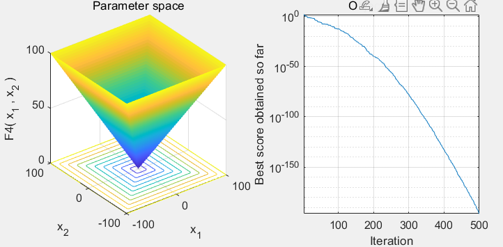
figure('Position',[269 240 660 290])
subplot(1,2,1);
func_plot(Function_name);
title('Parameter space')
xlabel('x_1');
ylabel('x_2');
zlabel([Function_name,'( x_1 , x_2 )'])
subplot(1,2,2);
semilogy(Convergence_curve)
hold on;
title('Objective space')
xlabel('Iteration');
ylabel('Best score obtained so far');
axis tight
grid on
box on
3.2 GTO优化CNN-LSTM超参数
看过我之前的博客都知道,任意优化算法来做超参数寻优是不需要懂优化算法的原理的,看3.1可知我们下载的这份GTO代码是用来做极小值寻优的就行。然后遵循以下步骤进行代码修改:
步骤1:知道要优化的参数与优化范围。显然就是第2节提到的11个参数。代码如下,首先改写lb与ub,然后初始化的时候注意除了学习率,其他的都是整数。并将原来里面的边界判断,改成了Bounds函数,方便在计算适应度函数值的时候转化成整数与小数。如果学习率的位置不在最后,而是在其他位置,就需要改随机初始化位置和Bounds函数与fitness函数里对应的地方,具体怎么改就不说了,很简单。
%% 人工大猩猩部队优化算法
function [Silverback,convergence_curve,process]=GTO(P_train,P_valid,T_train,T_valid)
%% 参数设置
%lb ub为寻优范围 第一列是学习率[0.0001-0.01]
%然后分别是训练次数 batchsize 卷积层1的卷积核数量、大小 池化层1的大小
%卷积层2的卷积核数量、大小  池化层1的大小 lstm层的节点数 全连接层的节点数
lb=[1e-4 10  8  1  1  1 1  1  1  1  1];
ub=[1e-2 100 64 20 10 5 20 10 5  50 200];
variables_no=length(lb);
pop_size=5;%种群数量
max_iter=10;%寻优代数

% initialize Silverback
Silverback=[];
Silverback_Score=inf;

%Initialize the first random population of Gorilla
for i=1:pop_size%随机初始化速度,随机初始化位置
    for j=1:variables_no
        X( i, j ) = (ub(j)-lb(j))*rand+lb(j);
    end
end

convergence_curve=zeros(max_iter,1);

for i=1:pop_size
    X(i,:) = Bounds( X(i,:), lb, ub );
    Pop_Fit(i)=fitness(X(i,:),P_train,P_valid,T_train,T_valid);
    if Pop_Fit(i)<Silverback_Score
        Silverback_Score=Pop_Fit(i);
        Silverback=X(i,:);
    end
end


GX=X(:,:);

%%  Controlling parameter

p=0.03;
Beta=3;
w=0.8;

%%Main loop
for It=1:max_iter

    a=(cos(2*rand)+1)*(1-It/max_iter);
    C=a*(2*rand-1);

    %% Exploration:

    for i=1:pop_size
        if rand<p
            GX(i,:) =(ub-lb).*rand(1,variables_no)+ub;
        else
            if rand>=0.5
                Z = unifrnd(-a,a,1,variables_no);
                H=Z.*X(i,:);
                GX(i,:)=(rand-a)*X(randi([1,pop_size]),:)+C.*H;
            else
                GX(i,:)=X(i,:)-C.*(C*(X(i,:)- GX(randi([1,pop_size]),:))+rand*(X(i,:)-GX(randi([1,pop_size]),:))); %ok ok

            end
        end
    end


    % Group formation operation
    for i=1:pop_size
        GX(i,:) = Bounds( GX(i,:), lb, ub );
        New_Fit= fitness(GX(i,:),P_train,P_valid,T_train,T_valid);
        if New_Fit<Pop_Fit(i)
            Pop_Fit(i)=New_Fit;
            X(i,:)=GX(i,:);
        end
        if New_Fit<Silverback_Score
            Silverback_Score=New_Fit;
            Silverback=GX(i,:);
        end
    end

    %% Exploitation:
    for i=1:pop_size
        if a>=w
            g=2^C;
            delta= (abs(mean(GX)).^g).^(1/g);
            GX(i,:)=C*delta.*(X(i,:)-Silverback)+X(i,:);
        else

            if rand>=0.5
                h=randn(1,variables_no);
            else
                h=randn(1,1);
            end
            r1=rand;
            GX(i,:)= Silverback-(Silverback*(2*r1-1)-X(i,:)*(2*r1-1)).*(Beta*h);

        end
    end

    % Group formation operation
    for i=1:pop_size
        GX(i,:) = Bounds( GX(i,:), lb, ub );

        New_Fit= fitness(GX(i,:),P_train,P_valid,T_train,T_valid);
        if New_Fit<Pop_Fit(i)
            Pop_Fit(i)=New_Fit;
            X(i,:)=GX(i,:);
        end
        if New_Fit<Silverback_Score
            Silverback_Score=New_Fit;
            Silverback=GX(i,:);
        end
    end
    It,Silverback_Score,Silverback
    convergence_curve(It)=Silverback_Score;
    process(It,:)=       Silverback;
end
end

function s = Bounds( s, Lb, Ub)
temp = s;
for i=1:length(s)
    if temp(:,i)>Ub(i) || temp(:,i)<Lb(i)
        temp(:,i) =rand*(Ub(i)-Lb(i))+Lb(i);
    end
    if i>1
        temp(:,i)=round(temp(:,i));%除了学习率 其他的都是整数
    end
end
s = temp;
end
步骤2:知道优化的目标。优化的目标是提高的网络的准确率,而GTO代码我们这个代码是最小值优化的,所以我们的目标可以是最小化CNN-LSTM的预测误差。预测误差具体是,测试集(或验证集)的预测值与真实值之间的均方差。
步骤3:构建适应度函数。通过步骤2我们已经知道优化的目标,即采用GTO去找11个值,用这11个值构建的CNN-LSTM网络,具备误差最小化。观察下面的代码,首先我们将GTO的值传进来,然后转成需要的11个值,然后构建网络,训练集训练、测试集预测,计算预测值与真实值的mse,将mse作为结果传出去作为适应度值。
function fit=fitness(x,P_train,P_valid,T_train,T_valid)
lr=x(1);
epochs=x(2);
miniBatchSize = x(3);
kernel1_num=x(4);
kernel1_size=x(5);
pool1_size=x(6);
kernel2_num=x(7);
kernel2_size=x(8);
pool2_size=x(9);
lstm_node=x(10);
fc_node=x(11);

rng(0)
input_size=[size(P_train{1}) 1];
output_size=size(T_train,2);
layers = [
    sequenceInputLayer(input_size,"Name","sequence")
    sequenceFoldingLayer("Name","seqfold")

    convolution2dLayer([kernel1_size kernel1_size],kernel1_num,"Name","conv_1","Padding","same")
    reluLayer("Name","relu_1")
    averagePooling2dLayer([1 pool1_size],"Name","avgpool2d_1")

    convolution2dLayer([kernel2_size kernel2_size],kernel2_num,"Name","conv_2","Padding","same")
    reluLayer("Name","relu_2")
    averagePooling2dLayer([1 pool2_size],"Name","avgpool2d_2")

    sequenceUnfoldingLayer("Name","sequnfold")
    flattenLayer("Name","flatten")
    lstmLayer(lstm_node,"Name","lstm",'OutputMode','last')
    fullyConnectedLayer(fc_node,"Name","fc")
    reluLayer("Name","relu_3")
    fullyConnectedLayer(output_size,"Name","out")
    regressionLayer("Name","regressionoutput")];
lgraph = layerGraph(layers);
lgraph = connectLayers(lgraph,"seqfold/miniBatchSize","sequnfold/miniBatchSize");

options = trainingOptions('adam', ...
    'MiniBatchSize',miniBatchSize, ...
    'MaxEpochs',epochs, ...
    'InitialLearnRate',lr,...
    'LearnRateSchedule','piecewise',...
    'LearnRateDropFactor',1,...
    'Shuffle','every-epoch', ...
    'Verbose',0);

[net,~] = trainNetwork(P_train,T_train,lgraph,options);
YPred1=predict(net,P_valid);
[m,n]=size(T_valid);
real=reshape(T_valid,[1,m*n]);
pred=reshape(YPred1,[1,m*n]);
fit =mse(real-pred);

% 以mse为适应度函数,优化算法目的就是找到一组超参数 使网络的mse最低
rng((100*sum(clock)))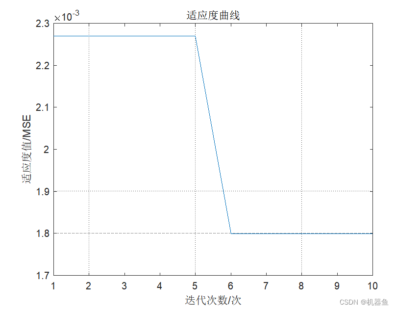
3.3 主程序
以下是调用上面这个优化算法的主程序,如下:
clc;clear;close all;format compact;format short
%%
data=xlsread('电荷数据.csv','B2:CX376');
%负荷数据--每天96各负荷值,气象数据 最高温度℃ 最低温度℃ 平均温度℃ 相对湿度(平均) 降雨量(mm)
power=data(:,1:96);
weather=data(:,97:end);
% 归一化 或者 标准化 看哪个效果好
method=@mapminmax;% mapstd mapminmax
[x1,mappingx1]=method(power');
[x2,mappingx2]=method(weather');
data=[x1' x2'];
% 前steps天steps*101 为输入,来预测未来一天的96负荷值 为输出
steps=10;
samples=size(data,1)-steps;%样本数
for i=1:samples
input{i,:}=data(i:i+steps-1,:);
output(i,:)=data(i+steps,1:96);
end
%% 数据划分 8:1:1划分训练集、验证集、测试集
n_samples=size(input,1);
n=1:n_samples;
m1=round(0.8*n_samples);
m2=round(0.9*n_samples);
Train_X=input(n(1:m1));
Train_Y=output(n(1:m1),:);
Val_X=input(n(m1+1:m2));
Val_Y=output(n(m1+1:m2),:);
Ttest_X=input(n(m2+1:end));
Ttest_Y=output(n(m2+1:end),:);
%% 参数优化
optimization=0;%是否重新优化
if optimization==1
[x ,fit_gen,process]=GTO(Train_X,Val_X,Train_Y,Val_Y);
save result/optim_result x fit_gen process
else
load result/optim_result
end
figure
plot(fit_gen)
grid on
title('适应度曲线')
xlabel('迭代次数/次')
ylabel('适应度值/MSE')
%% 网络搭建
lr=x(1)
epochs=x(2)
miniBatchSize = x(3)
kernel1_num=x(4)
kernel1_size=x(5)
pool1_size=x(6)
kernel2_num=x(7)
kernel2_size=x(8)
pool2_size=x(9)
lstm_node=x(10)
fc_node=x(11)
rng(0)
input_size=[size(Train_X{1}) 1];
output_size=size(Train_Y,2);
layers = [
sequenceInputLayer(input_size,"Name","sequence")
sequenceFoldingLayer("Name","seqfold")
convolution2dLayer([kernel1_size kernel1_size],kernel1_num,"Name","conv_1","Padding","same")
reluLayer("Name","relu_1")
averagePooling2dLayer([1 pool1_size],"Name","avgpool2d_1")
convolution2dLayer([kernel2_size kernel2_size],kernel2_num,"Name","conv_2","Padding","same")
reluLayer("Name","relu_2")
averagePooling2dLayer([1 pool2_size],"Name","avgpool2d_2")
sequenceUnfoldingLayer("Name","sequnfold")
flattenLayer("Name","flatten")
lstmLayer(lstm_node,"Name","lstm",'OutputMode','las')
fullyConnectedLayer(fc_node,"Name","fc")
reluLayer("Name","relu_3")
fullyConnectedLayer(output_size,"Name","out")
regressionLayer("Name","regressionoutput")];
lgraph = layerGraph(layers);
lgraph = connectLayers(lgraph,"seqfold/miniBatchSize","sequnfold/miniBatchSize");
figure
plot(lgraph)
title("模型结构")
options = trainingOptions('adam', ...
'MiniBatchSize',miniBatchSize, ...
'MaxEpochs',epochs, ...
'InitialLearnRate',lr,...
'LearnRateSchedule','piecewise',...
'LearnRateDropFactor',1,...
'Shuffle','every-epoch', ...
'ValidationData',{Val_X,Val_Y}, ...
'Verbose',1);
train_again=0;% 为1就代码重新训练模型,为0就是调用训练好的网络
if train_again==1
[net,traininfo] = trainNetwork(Train_X,Train_Y,lgraph,options);
save result/cnn_lstm_net2 net traininfo
else
load result/cnn_lstm_net2
end
figure
plot(traininfo.TrainingLoss);
grid on
title('CNN-LSTM');
xlabel('训练次数');
ylabel('损失值');
%% 预测,
YPred1=predict(net,Ttest_X);
YPred1=method('reverse',YPred1',mappingx1);
Ytest1=method('reverse',Ttest_Y',mappingx1);
[m,n]=size(Ytest1);
real=reshape(Ytest1,[1,m*n]);
pred=reshape(YPred1,[1,m*n]);
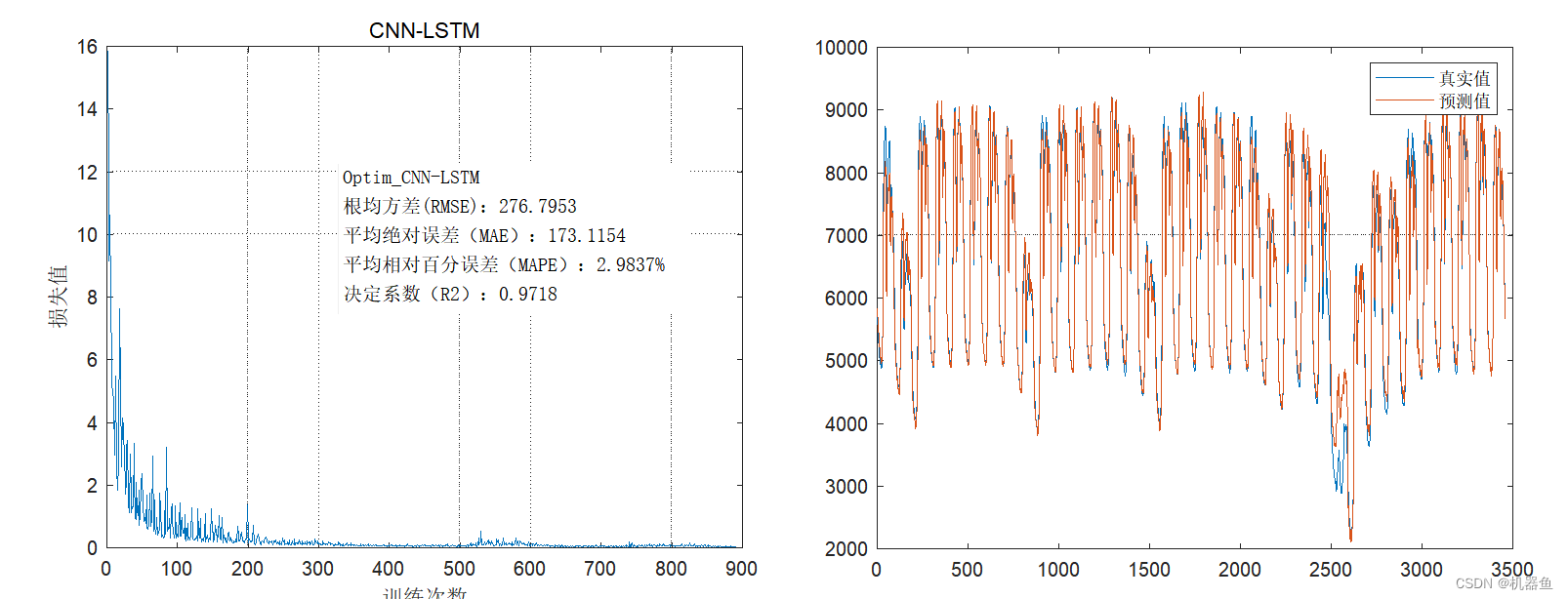
result(real,pred,'Optim_CNN-LSTM')
save result/optim_cnn_lstm_result real pred
figure
plot(real)
hold on;grid on
plot(pred)
legend('真实值','预测值')
4 结语
优化网络超参数的格式都是这样的!只要会改一种,那么随便拿一份能跑通的优化算法,在不管原理的情况下,都能用来优化网络的超参数。
更多内容【点击专栏】目录,您的点赞、关注、收藏是我更新【MATLAB神经网络1000个案例分析】的动力。


 741
741

 被折叠的 条评论
为什么被折叠?
被折叠的 条评论
为什么被折叠?
 到【灌水乐园】发言


