【吴恩达机器学习】第三周课程精简笔记——对数几率回归和正则化

Logistic Regression（对数几率回归/逻辑回归）

1. Classification and Representation（分类和表示）

（1）Classification

To attempt classification, one method is to use linear regression and map all predictions greater than 0.5 as a 1 and all less than 0.5 as a 0. However, this method doesn’t work well because classification is not actually a linear function.

The classification problem is just like the regression problem, except that the values we now want to predict take on only a small number of discrete values.For now, we will focus on the binary classification problem in which y can take on only two values, 0 and 1. (Most of what we say here will also generalize to the multiple-class case.)

---

想要分类，一种方法是使用线性回归，将所有大于0.5的预测都映射为1，所有小于0.5的预测都映射为0。然而，这种方法并不能很好地工作，因为分类实际上不是一个线性函数。

除了我们现在想要预测的值只取少量的离散值这一特点以外，分类问题就像回归问题一样。现在，我们将关注二元分类问题，在这个问题中，y只能取两个值，0和1。(我们在这里所说的大部分内容也适用于多类情况。)

（2）Hypothesis Representation（假设表示）

We could approach the classification problem ignoring the fact that y is discrete-valued, and use our old linear regression algorithm to try to predict y given x. However, it is easy to construct examples where this method performs very poorly. Intutitively, it also doesn’t make sense for $h_{\theta }(x)$ to take values larger than 1 or smaller than 0 when we know that y ∈ {0, 1}. To fix this, let’s change the form for our hypothesis $h_{\theta }(x)$ to satisfy $0\le h_{\theta }(x)\le 1$. This is accomplished by plugging ${\theta }^{T}x$ into the Logistic Function.

Our new form uses the “Sigmoid Function,” also called the “Logistic Function”:
$$\begin{array}{rl}{h}_{\theta }(x)& =g({\theta }^{T}x)\\ g(z)& =\frac{1}{1+e^{-z}}\\ z& ={\theta }^{T}x\end{array}$$

The following image shows us what the sigmoid function looks like:

The function g(z), shown here, maps any real number to the (0, 1) interval, making it useful for transforming an arbitrary-valued function into a function better suited for classification.
$$\begin{array}{rl}& h_{\theta }(x)=P(y=1|x;\theta )=1-P(y=0|x;\theta )\\ & P(y=0|x;\theta )+P(y=1|x;\theta )=1\end{array}$$

$h_{\theta }(x)$ will give us the probability that our output is 1. For example, $h_{\theta }(x)=0.7$ gives us a probability of 70% that our output is 1. Our probability that our prediction is 0 is just the complement of our probability that it is 1 (e.g. if probability that it is 1 is 70%, then the probability that it is 0 is 30%).

---

我们可以忽略y是离散值这一事实来处理分类问题，并使用我们上一周使用的线性回归算法来尝试在给定x时预测y的值。然而，很容易构造例子来证明出这种方法的性能非常差。直观地说，当我们知道 y∈{0,1} 时，对于$h_{}(x)$取大于1或小于0的值也没有意义。 为了解决这个问题，让我们改变假设 $h_{}(x)$ 的形式来满足 $0\le h_{}(x)\le 1$ 。 这是通过将 ${\theta }^{T}x$ 代入Logistic函数来完成的。

我们的新形式使用了“Sigmoid函数”，也称为“Logistic函数”:
$$\begin{array}{rl}{h}_{\theta }(x)& =g({\theta }^{T}x)\\ g(z)& =\frac{1}{1+e^{-z}}\\ z& ={\theta }^{T}x\end{array}$$

下面的图像展示了s形函数的样子:

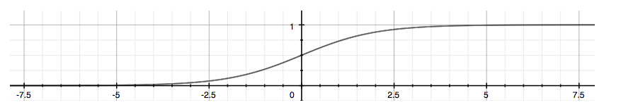
如图所示，函数g(z)将任意实数映射到(0,1)区间，这使得它可以将任意值函数转换为更适合分类的函数。
$$\begin{array}{rl}& h_{\theta }(x)=P(y=1|x;\theta )=1-P(y=0|x;\theta )\\ & P(y=0|x;\theta )+P(y=1|x;\theta )=1\end{array}$$
$h_{\theta }(x)$ 给出了输出为1时的概率。 例如，$h_{}(x)=0.7$ 表示输出为1的概率为70%。 我们预测结果为0的概率是预测结果为1的概率的补充（例如，如果预测结果为1的概率是70%，那么预测结果为0的概率是30% ）。

（3）Decision Boundary（决策边界）

1）Logistic regression

Remember：
$$\begin{gathered} z=0,e^0=1\Rightarrow g(z)=\frac{1}{2} \\ z\to \infty ,e^{-\infty }\to 0\Rightarrow g(z)=1 \\ z\to -\infty ,e^{\infty }\to \infty \Rightarrow g(z)=0 \end{gathered}$$

2）Decision Boundary

3）Non-Linear decision boundaries

2. Logistic Regression Model

（1）Cost Function

We cannot use the same cost function that we use for linear regression because the Logistic Function will cause the output to be wavy, causing many local optima. In other words, it will not be a convex function.

Instead, our cost function for logistic regression looks like:

$$\begin{array}{rl}& J(\theta )=\frac{1}{m}\sum _{i=1}^{m}Cost(h_{\theta }(x^{(i)}),y^{(i)})\\ & Cost(h_{\theta }(x),y)=-log(h_{\theta }(x))ify=1\\ & Cost(h_{\theta }(x),y)=-log(1-h_{\theta }(x))ify=0\end{array}$$

When y = 1, we get the following plot for $J(\theta )$ vs $h_{\theta }(x)$：

If our correct answer ‘y’ is 1, then the cost function will be 0 if our hypothesis function outputs 1. If our hypothesis approaches 0, then the cost function will approach infinity.

Similarly, when y = 0, we get the following plot for $J(\theta )$ vs $h_{\theta }(x)$:

If our correct answer ‘y’ is 0, then the cost function will be 0 if our hypothesis function also outputs 0. If our hypothesis approaches 1, then the cost function will approach infinity.

---

我们不能使用与线性回归相同的成本函数，因为Logistic函数会导致输出波动，导致许多局部最优值。 换句话说，它不是一个凸函数。

相反，我们的对数几率回归的代价函数是这样的：
$$\begin{array}{rl}& J(\theta )=\frac{1}{m}\sum _{i=1}^{m}Cost(h_{\theta }(x^{(i)}),y^{(i)})\\ & Cost(h_{\theta }(x),y)=-log(h_{\theta }(x))ify=1\\ & Cost(h_{\theta }(x),y)=-log(1-h_{\theta }(x))ify=0\end{array}$$

当y = 1时，我们得到$J(\Theta )$ vs $h(x)$的如下图：

当我们的正确答案y是1，那么如果假设函数输出1代价函数就是0。 如果我们的假设趋于0，那么代价函数将趋于无穷。

类似地，当y = 0时，我们得到$J(\theta )$ vs $h_{\theta }(x)$的下图：

当我们的正确答案y是0，如果我们的假设函数输出也是0，那么代价函数就是0。 如果我们的假设趋于1，那么代价函数将趋于无穷。

（2）Simplified Cost Function and Gradient Descent（简化代价函数和梯度下降）

We can compress our cost function’s two conditional cases into one case:
$$Cost(h_{\theta }(x),y)=-ylog(h_{\theta }(x))-(1-y)log(1-h_{\theta }(x))$$
We can fully write out our entire cost function as follows:
$$J(\theta )=-\frac{1}{m}\sum _{i=1}^m[y^{(i)}log(h_{\theta }(x^i))+(1-y^{(i)})log(1-h_{\theta }(x^i))]$$
A vectorized implementation is:
$$\begin{array}{rl}& h=g({\theta }^{T}X)\\ & J(\theta )=\frac{1}{m}(-y^{T}log(h)-(1-y{)}^{T}log(1-h))\end{array}$$
We can work out the derivative part using calculus to get:
R e p e a t { θ j : = θ j − α m ∑ i = 1 m ( h θ ( x ( i ) − y ( i ) ) x j ( i ) } \begin{aligned} &Repeat \{ \\ &\theta_j := \theta_j - \frac{\alpha}{m} \sum_{i=1}^{m} (h_\theta(x^{(i)}-y^{(i)})x_j^{(i)} \\ \} \end{aligned} }​Repeat{θj​:=θj​−mα​i=1∑m​(hθ​(x(i)−y(i))xj(i)​​

Notice that this algorithm is identical to the one we used in linear regression. We still have to simultaneously update all values in theta.

A vectorized implementation is:
$$\theta :=\theta -\frac{\alpha }{m}{X}^T(g({\theta }^{T}X)-\vec{y})$$

This cost function can be derived from statistics using the principle of maximum likelihood estimation which is an idea in statistics for how to efficiently find parameters theta for different models. And it also has a nice property that it is a convex.

---

我们可以将代价函数的两个条件情形压缩为一个情形：
$$Cost(h_{\theta }(x),y)=-ylog(h_{\theta }(x))-(1-y)log(1-h_{\theta }(x))$$
我们可以完全写出整个代价函数如下：
$$J(\theta )=-\frac{1}{m}\sum _{i=1}^m[y^{(i)}log(h_{\theta }(x^i))+(1-y^{(i)})log(1-h_{\theta }(x^i))]$$
一个向量化的实现是：
$$h=g({\theta }^{T}X)J(\theta )=\frac{1}{m}(-y^{T}log(h)-(1-y{)}^{T}log(1-h))$$
我们可以用微积分计算出导数部分，得到:
R e p e a t { θ j : = θ j − α m ∑ i = 1 m ( h θ ( x ( i ) − y ( i ) ) x j ( i ) } \begin{aligned} Repeat &\{ \\ &\theta_j := \theta_j - \frac{\alpha}{m} \sum_{i=1}^{m} (h_\theta(x^{(i)}-y^{(i)})x_j^{(i)} \\ \} \end{aligned} Repeat}​{θj​:=θj​−mα​i=1∑m​(hθ​(x(i)−y(i))xj(i)​​
注意，这个算法与我们在线性回归中使用的算法相同。 我们仍然需要同时更新所有的值。

一个向量化的实现是：
$$\theta :=\theta -\frac{\alpha }{m}{X}^T(g({\theta }^{T}X)-\vec{y})$$
这个代价函数可以用极大似然估计准则从统计中推导出来，极大似然估计是统计学中的一种思想，用来有效地为不同的模型找到参数 $\theta$。 它还有一个很好的性质，那就是它估计出的函数是凸函数。

（3）Advanced Optimization（高级优化）

“Conjugate gradient”, “BFGS”, and “L-BFGS” are more sophisticated, faster ways to optimize θ that can be used instead of gradient descent.

Advantages:
No need to manually pick $\alpha$, instead have a clever inner-loop.
It is often faster than gradient descent

Disadvantages:
More Complex.

We suggest that you should not write these more sophisticated algorithms yourself (unless you are an expert in numerical computing) but use the libraries instead, as they’re already tested and highly optimized. Octave provides them.

---

“共轭梯度法”、“BFGS法”和“L-BFGS法”是一种比梯度下降法更复杂、更快速的θ优化方法。

优点：
不需要手动选择$\alpha$，而是有一个更智能的内部循环。
它通常比梯度下降快。

缺点：
更加复杂。

我们建议您不要自己编写这些更复杂的算法(除非您是数值计算方面的专家)，而是使用库，因为它们已经经过了测试和高度优化。

3. Multiclass Classification：One-vs-all

Now we will approach the classification of data when we have more than two categories. Instead of y = {0,1} we will expand our definition so that y = {0,1…n}.

Since y = {0,1…n}, we divide our problem into n+1 (+1 because the index starts at 0) binary classification problems; in each one, we predict the probability that ‘y’ is a member of one of our classes.

One-vs-all: Train a logistic regression classifier $h_{\theta }^{(i)}(x)$ for each class i to predict the probability that y = i.

On a new input x, to make a prediction pick the class i that maximizes.
$$\underset{i}{\max }{h}_{\theta }^{(i)}(x)$$

---

现在，当我们有两个以上的类别时，我们将处理数据的分类。 我们将扩展定义，使y ={0,1…n}，而不是y ={0,1}。

因为y ={0,1… N}，我们将问题划分为N +1(+1是因为索引从0开始)二元分类问题; 在每个类中，我们预测“y”是我们类中的一个成员的概率。

一对多: 训练一个逻辑回归分类器 $h_{\theta }^{(i)}(x)$ 为每个类 i 预测 y = i 的概率 。

对于一个新的输入x，为了做出预测，选择类 i 使 $h_{\theta }^{(i)}(x)$ 最大化。
$$\underset{i}{\max }{h}_{\theta }^{(i)}(x)$$

4. Solving the Problem of Overfitting

（1）The Problem of Overfitting

Without formally defining what these terms mean, we’ll say the figure on the left shows an instance of underfitting—in which the data clearly shows structure not captured by the model—and the figure on the right is an example of overfitting.

Underfitting, or high bias, is when the form of our hypothesis function h maps poorly to the trend of the data. It is usually caused by a function that is too simple or uses too few features. At the other extreme, overfitting, or high variance, is caused by a hypothesis function that fits the available data but does not generalize well to predict new data. It is usually caused by a complicated function that creates a lot of unnecessary curves and angles unrelated to the data.

This terminology is applied to both linear and logistic regression. There are two main options to address the issue of overfitting:

1. Reduce the number of features:

• Manually select which features to keep.
• Use a model selection algorithm (studied later in the course).

2. Regularization

• Keep all the features, but reduce the magnitude of parameters ${\theta }_j$ .
• Regularization works well when we have a lot of slightly useful features.

---

在没有正式定义这些术语含义的情况下，我们会说左边的图显示了一个欠拟合的例子——其中数据清楚地显示了模型没有捕获到的结构——而右边的图则是一个过拟合的例子。

欠拟合或高偏倚，指当我们的假设函数h的形式不能很好的映射出数据的趋势。它通常是由于一个函数太简单或使用特征太少。在另一个极端，过度拟合或高方差，指由于一个假设函数能很好的你和现有的数据，但不能很好地泛化以预测新的数据。这通常是由一个复杂的函数引起的，它会产生大量与数据无关的不必要的曲线和角度。

这个术语既适用于线性回归，也适用于逻辑回归。 解决过拟合问题有两种主要方法：

1. 减少特征的数量:

• 手动选择要保留的特征。
• 使用模型选择算法（稍后将在课程中学习）。

2. 正则化

• 保留所有的特性，但减少参数 ${\theta }_j$ 的数量级。
• 当我们有很多稍微有用的特性时，正则化工作得很好。

（2）Cost Function

If we have overfitting from our hypothesis function, we can reduce the weight that some of the terms in our function carry by increasing their cost.

Say we wanted to make the following function more quadratic:
${\theta }_0+{\theta }_{1}x+{\theta }_2{x}^2+{\theta }_3{x}^3+{\theta }_4{x}^4$

We’ll want to eliminate the influence of ${\theta }_3{x}^3$ and ${\theta }_4{x}^4$.Without actually getting rid of these features or changing the form of our hypothesis, we can instead modify our cost function:
$$\underset{\theta }{\min }\frac{1}{2m}\sum _{i=1}^m(h_{\theta }(x^{(i)})-y^{(i)}{)}^2+1000\cdot {\theta }_3^2+1000\cdot {\theta }_4^2$$

We’ve added two extra terms at the end to inflate the cost of ${\theta }_3$ and ${\theta }_4$. Now, in order for the cost function to get close to zero, we will have to reduce the values of ${\theta }_3$ and ${\theta }_4$ to near zero. This will in turn greatly reduce the values of ${\theta }_3{x}^3$ and ${\theta }_4{x}^4$ in our hypothesis function. As a result, we see that the new hypothesis (depicted by the pink curve) looks like a quadratic function but fits the data better due to the extra small terms ${\theta }_3{x}^3$ and ${\theta }_4{x}^4$.

We could also regularize all of our theta parameters in a single summation as:
$$\underset{\theta }{\min }\frac{1}{2m}\sum _{i=1}^m(h_{\theta }(x^{(i)})-y^{(i)}{)}^2+\lambda \sum _{j=1}^n{\theta }_j^2$$

The λ, or lambda, is the regularization parameter. It determines how much the costs of our theta parameters are inflated.

Using the above cost function with the extra summation, we can smooth the output of our hypothesis function to reduce overfitting. If lambda is chosen to be too large, it may smooth out the function too much and cause underfitting.

If ${\theta }_1$≈0 , ${\theta }_2$≈0 , ${\theta }_3$≈0 , ${\theta }_4$≈0, $h_{\theta }(x)$ is equail ${\theta }_0$ which is going to be a flat straight line

---

如果我们的假设函数过拟合，我们可以通过增加一些项的代价来减少函数中这些项的权重。

假设我们想让以下函数保留更多次方：
${\theta }_0+{\theta }_{1}x+{\theta }_2{x}^2+{\theta }_3{x}^3+{\theta }_4{x}^4$

我们要消除 ${\theta }_3{x}^3$ 和 ${\theta }_4{x}^4$ 的影响。在不去除这些特征或改变假设形式的情况下，我们可以修改我们的代价函数：
$$\underset{\theta }{\min }\frac{1}{2m}\sum _{i=1}^m(h_{\theta }(x^{(i)})-y^{(i)}{)}^2+1000\cdot {\theta }_3^2+1000\cdot {\theta }_4^2$$

我们在式子末尾增加了额外的两项，以提高 ${\theta }_3$ 和 ${\theta }_4$ 的代价。现在，为了使代价函数接近于零，我们必须将 ${\theta }_3$ 和 ${\theta }_4$ 的值降低到接近于零。 这将反过来将会使我们的假设函数中的 ${\theta }_3{x}^3$ 和 ${\theta }_4{x}^4$ 的值大大减少。 结果，我们看到新的假设（用粉色曲线表示）看起来像一个二次函数，由于有额外的小项 ${\theta }_3{x}^3$ 和 ${\theta }_4{x}^4$，故该函数能更好的拟合数据。

我们也可以在一个求和（函数）中正则化所有的参数 $\theta$：
$$\underset{\theta }{\min }\frac{1}{2m}\sum _{i=1}^m(h_{\theta }(x^{(i)})-y^{(i)}{)}^2+\lambda \sum _{j=1}^n{\theta }_j^2$$

λ或lambda是正则化参数，它决定了参数膨胀代价的大小。

使用上面的代价函数和额外的求和（函数），我们可以平滑我们的假设函数的输出，以减少过拟合。 如果选择的lambda太大，可能会使函数过于平滑，导致欠拟合。

如果 ${\theta }_1$≈0 , ${\theta }_2$≈0 , ${\theta }_3$≈0 , ${\theta }_4$≈0, $h_{\theta }(x)$ = ${\theta }_0$，会成为一条平坦的直线。

（3）Regularized Linear Regression

Gradient Descent
We will modify our gradient descent function to separate out ${\theta }_0$ from the rest of the parameters because we do not want to penalize ${\theta }_0$.
​ R e p e a t { θ 0 : = θ 0 − α 1 m ∑ i = 1 m ( h θ ( x ( i ) ) − y ( i ) ) x 0 ( j ) θ j : = θ j − α [ ( 1 m ∑ i = 1 m ( h θ ( x ( i ) ) − y ( i ) ) x j ( j ) ) + λ m θ j ] j ∈ { 1 , 2 , 3... n } } \begin{aligned} Repeat& \{ \\ &\theta_0 := \theta_0 - \alpha \frac{1}{m} \sum_{i=1}^m(h_\theta(x^{(i)})-y^{(i)})x_0^{(j)} \\ &\theta_j := \theta_j - \alpha[ (\frac{1}{m} \sum_{i=1}^m(h_\theta(x^{(i)})-y^{(i)})x_j^{(j)}) + \frac{\lambda}{m} \theta_j ] \qquad j \in \{1,2,3...n\} \\ \} \end{aligned} Repeat}​{θ0​:=θ0​−αm1​i=1∑m​(hθ​(x(i))−y(i))x0(j)​θj​:=θj​−α[(m1​i=1∑m​(hθ​(x(i))−y(i))xj(j)​)+mλ​θj​]j∈{1,2,3...n}​

The term $\frac{\lambda }{m}{\theta }_j$ performs our regularization. With some manipulation our update rule can also be represented as:
${\theta }_j:={\theta }_j(1-\alpha \frac{\lambda }{m})-\alpha \frac{1}{m}{\sum }_{i=1}^m(h_{\theta }(x^{(i)})-y^{(i)})x_j^{(i)}$

The first term in the above equation, $1-\alpha \frac{\lambda }{m}$ will always be less than 1. Intuitively you can see it as reducing the value of ${\theta }_j$ by some amount on every update. Notice that the second term is now exactly the same as it was before.

Normal Equation
To add in regularization, the equation is the same as our original, except that we add another term inside the parentheses:
$$\begin{gathered} \theta =(X^{T}X+\lambda \cdot L{)}^{-1}{X}^{T}y \\ whereL=\left[\begin{array}{ccccc}0& & & & \\ & 1& & & \\ & & 1& & \\ & & & \ddots & \\ & & & & 1\end{array}\right] \end{gathered}$$
L is a matrix with 0 at the top left and 1’s down the diagonal, with 0’s everywhere else. It should have dimension (n+1)×(n+1). Intuitively, this is the identity matrix (though we are not including $x_0$), multiplied with a single real number λ.

Recall that if m < n, then $X^{T}X$ is non-invertible. However, when we add the term λ⋅L, then $X^{T}X+\lambda \cdot L$ becomes invertible. This matrix will be invertible and will not be singular.

---

梯度下降法
我们将修改梯度下降函数，将 ${\theta }_0$ 从其他参数中分离出来，因为我们不想惩罚 ${\theta }_0$ 。
​ R e p e a t { θ 0 : = θ 0 − α 1 m ∑ i = 1 m ( h θ ( x ( i ) ) − y ( i ) ) x 0 ( j ) θ j : = θ j − α [ ( 1 m ∑ i = 1 m ( h θ ( x ( i ) ) − y ( i ) ) x j ( j ) ) + λ m θ j ] j ∈ { 1 , 2 , 3... n } } \begin{aligned} Repeat& \{ \\ &\theta_0 := \theta_0 - \alpha \frac{1}{m} \sum_{i=1}^m(h_\theta(x^{(i)})-y^{(i)})x_0^{(j)} \\ &\theta_j := \theta_j - \alpha[ (\frac{1}{m} \sum_{i=1}^m(h_\theta(x^{(i)})-y^{(i)})x_j^{(j)}) + \frac{\lambda}{m} \theta_j ] \qquad j \in \{1,2,3...n\} \\ \} \end{aligned} Repeat}​{θ0​:=θ0​−αm1​i=1∑m​(hθ​(x(i))−y(i))x0(j)​θj​:=θj​−α[(m1​i=1∑m​(hθ​(x(i))−y(i))xj(j)​)+mλ​θj​]j∈{1,2,3...n}​

$\frac{\lambda }{m}{\theta }_j$ 执行我们的正则化。 通过一些操作，我们的更新规则也可以表示为：
${\theta }_j:={\theta }_j(1-\alpha \frac{\lambda }{m})-\alpha \frac{1}{m}{\sum }_{i=1}^m(h_{\theta }(x^{(i)})-y^{(i)})x_j^{(i)}$

上式的第一项 $1-\alpha \frac{\lambda }{m}$ 总是小于1。 直观地，您可以看到它在每次更新时减少了 ${\theta }_j$ 的值。 注意，第二项现在和以前完全一样。

正规方程法
在正则化中，方程和原来的方程一样，除了我们在括号中添加了另一项:
$$\begin{gathered} \theta =(X^{T}X+\lambda \cdot L{)}^{-1}{X}^{T}y \\ whereL=\left[\begin{array}{ccccc}0& & & & \\ & 1& & & \\ & & 1& & \\ & & & \ddots & \\ & & & & 1\end{array}\right] \end{gathered}$$
L是一个矩阵，0在左上角，1在对角线上，其他地方都是0。 它的维数应该是(n+1)×(n+1)。 直观地说，这是单位矩阵（尽管不包括$x_0$）乘以一个实数λ。

回想一下，如果m < n，那么$X^{T}X$是不可逆的。 然而，当我们添加λ⋅L项时，则$X^{T}X+\lambda \cdot L$变为可逆项。这个矩阵是可逆的并且不是奇异的。

（4）Regularized Logistic Regression

We can regularize logistic regression in a similar way that we regularize linear regression. As a result, we can avoid overfitting. The following image shows how the regularized function, displayed by the pink line, is less likely to overfit than the non-regularized function represented by the blue line:

Cost Function
Recall that our cost function for logistic regression was:
$J(\theta )=-\frac{1}{m}{\sum }_{i=1}^m[y^{(i)}log(h_{\theta }(x^{(i)}))+(1-y^{(i)})log(1-h_{\theta }(x^{(i)}))]$

We can regularize this equation by adding a term to the end:
$J(\theta )=-\frac{1}{m}{\sum }_{i=1}^m[y^{(i)}log(h_{\theta }(x^{(i)}))+(1-y^{(i)})log(1-h_{\theta }(x^{(i)}))+\frac{\lambda }{2m}{\sum }_{i=1}^n{\theta }_j^2]$

The second sum, ${\sum }_{j=1}^n{\theta }_j^2$ means to explicitly exclude the bias term, ${\theta }_0$.I.e. the θ vector is indexed from 0 to n (holding n+1 values,${\theta }_0$ through ${\theta }_n$), and this sum explicitly skips ${\theta }_0$ , by running from 1 to n, skipping 0. Thus, when computing the equation, we should continuously update the two following equations:

Advanced optimization

---

我们可以用正则化线性回归的方法来正则化逻辑回归。 因此，我们可以避免过度拟合。 下图显示了由粉色线显示的正则化函数是如何比由蓝色线表示的非正则化函数更不容易过拟合的。
代价函数
回想一下，logistic回归的代价函数是:
$J(\theta )=-\frac{1}{m}{\sum }_{i=1}^m[y^{(i)}log(h_{\theta }(x^{(i)}))+(1-y^{(i)})log(1-h_{\theta }(x^{(i)}))]$

我们可以正则化这个方程，方法是在最后加一项:
$J(\theta )=-\frac{1}{m}{\sum }_{i=1}^m[y^{(i)}log(h_{\theta }(x^{(i)}))+(1-y^{(i)})log(1-h_{\theta }(x^{(i)}))+\frac{\lambda }{2m}{\sum }_{i=1}^n{\theta }_j^2]$

第二项求和 ${\sum }_{j=1}^n{\theta }_j^2$ 意味着明确排除偏差项 ${\theta }_0$ 。向量 $\theta$ 的索引是从0到n(保留n+1个值，${\theta }_0$到${\theta }_n$)，这个很明显地跳过了 ${\theta }_0$，从（索引）1到n，跳过0。 因此，在计算方程时，我们需要不断更新以下两个方程：

高级优化

Exercise 2：对数几率回归和正则化

【吴恩达机器学习】Week3 编程作业——对数几率回归和正则化