机器学习——支持向量机

风月雅颂

于 2023-12-27 14:25:15 发布

阅读量2.3k

点赞数 33

分类专栏：机器学习-基于sklearn 文章标签：机器学习支持向量机人工智能 python

本文链接：https://blog.csdn.net/qq_41566819/article/details/135239712

版权

机器学习-基于sklearn 专栏收录该内容

25 篇文章 1 订阅

订阅专栏

【说明】文章内容来自《机器学习——基于sklearn》，用于学习记录。若有争议联系删除。

1、简介

支持向量机(support vector machine,SVM)是一类按监督学习方式对数据进行二元分类的广义线性分类器，其决策边界是对学习样本求解的最大边距超平面(maximum-marginhyperplane)。与逻辑回归和神经网络相比，支持向量机在学习复杂的非线性方程时提供了一种更清晰、更强大的方式。

1.1 算法思想

支持向量机(Support Vector Machine,SVM)的基本思想是在N维数据找到N-1维的超平面(hyperplane)作为分类的决策边界。确定超平面的规则是：找到离超平面最近的那些点，使它们与超平面的距离尽可能远。在图中，离超平面最近的实心点和空心点称为支持向量，超平面两侧的支持向量与超平面的距离之和称为间隔距离，即图中的2/Ilwll。间隔距离越大，分类的准确率越高。在图中，两条虚线称为决策边界。

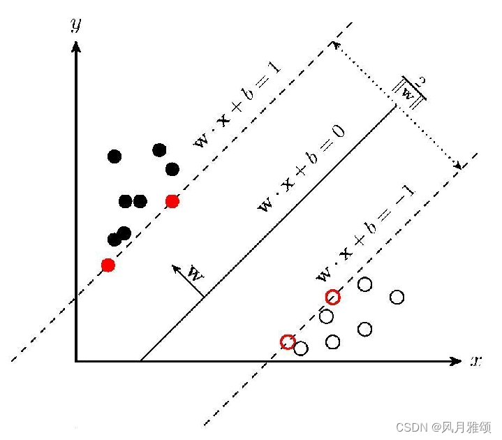
超平面可以用如下的线性方程来描述:

$wx + b = 0$
其中，w是超平面的法向量，定义了垂直于超平面的方向，b用于平移超平面。
支持向量机之所以成为目前最常用、效果最好的分类器之一，在小样本训练集上能够得到比其他算法更好的结果，原因就在于其优秀的泛化能力。但是，如果数据量很大(如垃圾邮件的分类检测），支持向量机的训练时间就会比较长。

1.2 支持向量机算法库

Sklearn 中支持向量机的算法库分为两类：一类是分类算法库，包括SVC、NuSVC和LinearSVC；另一类是回归算法库，包括svm、LinearSVR、svm.NuSVR、svm.SVR
在 SVC.NuSVC和 LinearSVC这3个分类算法库中，SVC和 NuSVC 差不多，区别仅在于两者对损失的度量方式不同；而LinearSVC 只用于线性分类，不支持各种从低维到高维的核函数，仅支持线性核函数，对线性不可分的数据不能使用。

2、核函数

核函数用于将非线性问题转化为线性问题。通过特征变换增加新的特征，使得低维空间中的线性不可分问题变为高维空间中的线性可分问题，进行升维变换。
SVC的语法如下:

SVC(kernel)

参数 kernel的取值有rbf、linear、 poly,代表不同的核函数。默认的rbf 代表径向基核函数(高斯核函数)，linear 代表线性核函数，poly 代表多项式核函数。

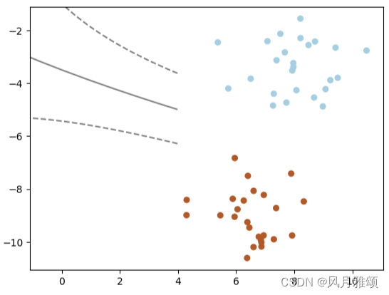
2.1 径向基核函数

径向基核函数通过高斯分布函数衡量样本之间的相似度，进而使样本线性可分。径向基核函数的kernel参数取值为rbf，格式如下:

SVC(kernel='rbf', C)

示例：

import numpy as np
import matplotlib.pyplot as plt
from sklearn import svm
from sklearn.datasets import make_blobs
#先创建50个数据点，将它们分为两类
x, y = make_blobs(n_samples = 50, centers = 2, random_state = 6)
#创建径向基核的支持向量机模型
clf_rbf = svm.SVC(kernel = 'rbf', C = 1000)
clf_rbf.fit(x, y)
#画数据点
plt.scatter(x[:,0], x[:,1], c= y, s = 30, cmap = plt.cm.Paired)
#建立图像坐标
ax = plt.gca()
xlim = ax.get_xlim()
ylim = ax.get_ylim()
xx = np.linspace(xlim[0], ylim[1], 30)
yy = np.linspace(ylim[0], ylim[1], 30)
YY, XX = np.meshgrid(yy, xx)
xy = np.vstack([XX.ravel(), YY.ravel()]).T
Z = clf_rbf.decision_function(xy).reshape(XX.shape)
#把分类的决定边界画出来
ax.contour(XX, YY, Z, colors = 'k', levels = [-1, 0, 1], alpha = 0.5, linestyles = ['--', '-', '--'])
ax.scatter(clf_rbf.support_vectors_[:, 0], clf_rbf.support_vectors_[:, 1], s = 100, linewidth = 1, facecolors = 'none')
plt.show()

【运行结果】

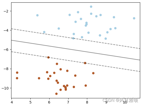
2.2 线性核函数

线性核函数(linear kernel)不通过核函数进行维度提升，仅在原始维度空间中寻求线性分类边界。线性核函数的kernel参数取值为linear,格式如下:

SVC(kernel='linear', C)

参数C为惩罚系数,用来控制损失函数的惩罚系数，类似于线性回归中的正则化系数。
C值越大，对误分类的惩罚越重，这样会使训练集在测试时准确率很高，但泛化能力弱，容易导致过拟合；C值越小，对误分类的惩罚越轻，容错能力和泛化能力强，但容易导致欠拟合。

线性核函数示例

import numpy as np
import matplotlib.pyplot as plt
from sklearn import svm
from sklearn.datasets import make_blobs
#先创建50个数据点，让它们分为两类
X, y = make_blobs(n_samples = 50, centers = 2, random_state = 6)
#创建一个线性核的支持向量机面模型
clf = svm.SVC(kernel= 'linear', C = 1000)
clf.fit(X,y)
#把数据点画出来
plt.scatter(X[:, 0], X[:, 1], c = y, s = 30, cmap = plt.cm.Paired)
#建立图像坐标
ax = plt.gca()#获取坐标轴信息
xlim = ax.get_xlim()
ylim = ax.get_ylim()
xx = np.linspace(xlim[0], xlim[1], 30)
yy = np.linspace(ylim[0], ylim[1], 30)
YY, XX = np.meshgrid(yy, xx)# meshgrid在二维平面将每一个x和每一个y分别对应起来，编织成栅格
xy = np.vstack([XX.ravel(), YY.ravel()]).T#ravel()将数组维度拉成一维数组,np.vstack在竖直方向上堆叠
z = clf.decision_function(xy).reshape(XX.shape)
#把分类的决策边界画出来contour绘制等高线函数
ax.contour(XX, YY, z, colors = 'k', levels = [-1,0,1], alpha = 0.5, linestyles = ['--','-','--'])
ax.scatter(clf.support_vectors_[:, 0], clf.support_vectors_[:, 1], s = 100, linewidth = 1, facecolors = 'none')
plt.show()

【运行结果】

2.3 多项式核函数

多项式核函数通过多项式函数增加原始样本特征的高次幂，把样本特征投射到高位空间。多项式核函数的kernel参数取值为ploy。格式如下：

SVC(kernel = 'ploy', degree = 3)

参数degree表示选择的多项式的最高幂次，默认为三次多项式。

from sklearn.svm import SVC
import numpy as np
X = np.array([[1,1],[1,2],[1,3],[1,4],[2,1],[2,2],[3,1],[4,1],[5,1],[5,2],[6,1],[6,2],[6,3],[6,4],[3,3],[3,4]
             ,[3,5],[4,3],[4,4],[4,5]])
Y = np.array([1] * 14 + [-1] * 6)
T = np.array([[0.5, 0.5], [1.5, 1.5], [3.5, 3.5], [4, 5.5]])
#X 为训练样本， Y为训练样本标签（1 和-1）， T为测试样本
svc = SVC(kernel = 'poly', degree = 2, gamma = 1, coef0 = 0)
svc.fit(X, Y)
pre = svc.predict(T)
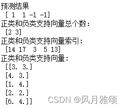
print('预测结果\n', pre)
print('正类和负类支持向量总个数：\n',svc.n_support_)
print("正类和负类支持向量索引:\n", svc.support_)
print("正类和负类支持向量:\n", svc.support_vectors_)

【运行结果】

3、参数调优

3.1 gamma参数

gamma用于控制核函数的影响范围，主要适用于使用径向基函数（RBF）或多项式核函数（Poly）。

对于RBF核函数，gamma参数定义了单个训练样本对模型的影响范围。较小的gamma值表示影响范围较大，样本之间的距离相对较远的特征也可能被考虑进来，从而使决策边界更加平滑。较大的gamma值表示影响范围较小，模型将更加关注每个训练样本的局部区域，可能会导致决策边界更加复杂和详细。

对于Poly核函数，gamma参数定义了特征空间中特征的相似度。较小的gamma值表示特征之间的相似度较高，从而产生更平滑的决策边界。较大的gamma值表示特征之间的相似度较低，可能导致更复杂的决策边界。

import sklearn.svm as svm
import matplotlib.pyplot as plt
from sklearn.datasets import load_wine
import numpy as np
def make_meshgrid(x, y, h = .02):
    x_min, x_max = x.min() - 1, x.max() + 1
    y_min, y_max = y.min() - 1, y.max() + 1
    xx, yy = np.meshgrid(np.arange(x_min, x_max, h), np.arange(y_min, y_max, h))
    return xx, yy
def plot_contours(ax, clf, xx, yy, **params):
    z = clf.predict(np.c_[xx.ravel(), yy.ravel()])
    z = z.reshape(xx.shape)
    out = ax.contourf(xx, yy, z, **params)
#使用酒的数据集
wine = load_wine()
#选取数据集的前两个特征
X = wine.data[:,:2]
y = wine.target
C = 1.0
models = (svm.SVC(kernel = 'rbf', gamma = 0.1, C = C),
         svm.SVC(kernel = 'rbf', gamma = 1,  C = C),
         svm.SVC(kernel = 'rbf', gamma = 10,  C = C))
models = (clf.fit(X, y) for clf in models)
titles = ('gamma = 0.1','gamma = 1', 'gamma = 10')
fig, sub = plt.subplots(1, 3, figsize = (10, 3))
#plt.subplots_adjust(wspace = 0.8, hspace = 0.2)
X0, X1 = X[:, 0], X[:, 1]
xx, yy = make_meshgrid(X0, X1)
for clf, title, ax in zip(models, titles, sub.flatten()):
    plot_contours(ax, clf, xx, yy, cmap = plt.cm.plasma, alpha = 0.8)
    ax.scatter(X0, X1, c = y, cmap = plt.cm.plasma, s = 20, edgecolors = 'k')
    ax.set_xlim(xx.min(), xx.max())
    ax.set_ylim(yy.min(), yy.max())
    ax.set_xlabel("Feature 0")
    ax.set_ylabel('Feature 1')
    ax.set_xticks(())
    ax.set_yticks(())
    ax.set_title(title)
plt.show()
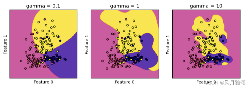
# 参数gamma分别取值为0.1.1和10。
# gamma值越小，径向基核直径越大,进入支持向量机的决策边界中的数据越多,决策边界越平滑，模型越简单;
# gamma值越大,支持向量机越倾向于把尽可能多的数据放到决策边界中,模型的复杂度越高。
# 所以,gamma值越小，模型越倾向于欠拟合;gamma值越大,模型倾向于过拟合。

【运行结果】

3.2 惩罚系数C

        C是惩罚系数，即对误差的宽容度,用于调节优化方向中的两个指标(间隔大小和分类准确度)的权重，表示对分错数据的惩罚力度。
        当C较大时，分错的数据就会较少,但是过拟合的情况会比较严重;
        当C较小时，容易出现欠拟合的情况。
        C越大，训练的迭代次数越大，训练时间越长。

from sklearn import datasets
from sklearn.model_selection import GridSearchCV
from sklearn.svm import SVC
from sklearn.model_selection import train_test_split
iris = datasets.load_iris()
x = iris.data[:,:2]
y = iris.target
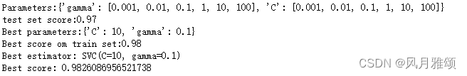
param_grid = {'gamma': [0.001, 0.01, 0.1, 1, 10, 100], 'C': [0.001, 0.01, 0.1, 1, 10, 100]}
print("Parameters:{}".format(param_grid))
grid_search = GridSearchCV(SVC(), param_grid, cv = 5)
x_train, x_test, y_train, y_test = train_test_split(iris.data, iris.target, random_state = 10)
grid_search.fit(x_train, y_train)
print("test set score:{:.2f}".format(grid_search.score(x_test, y_test)))
print('Best parameters:{}'.format(grid_search.best_params_))
print('Best score om train set:{:.2f}'.format(grid_search.best_score_))
print('Best estimator:',grid_search.best_estimator_)
print('Best score:',grid_search.best_score_)

【运行结果】

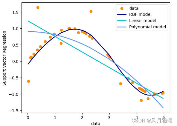
4、回归问题

支持向量机分类方法能推广到回归问题，称为支持向量回归。支持向量回归有3个版本：SVR、NuSVR和LinearSVR。

import numpy as np
from sklearn.svm import SVR
import matplotlib.pyplot as plt
#产生样本数据
x = np.sort(5*np.random.rand(40, 1), axis = 0)
y = np.sin(x).ravel()
#在目标值中增加噪声数据
y[::5] += 3*(0.5 -np.random.rand(8))
#估计器
svr_rbf = SVR(kernel = 'rbf', C = 1e3, gamma = 0.1)#径向基核函数
svr_lin = SVR(kernel = 'linear', C = 1e3)#线性核函数
svr_poly = SVR(kernel = 'poly', C = 1e3, degree = 2)#多项式核函数
y_rbf = svr_rbf.fit(x, y).predict(x)
y_lin = svr_lin.fit(x, y).predict(x)
y_poly = svr_poly.fit(x, y).predict(x)
lw = 2
plt.scatter(x, y, color = 'darkorange', label = 'data')
plt.plot(x, y_rbf, color = 'navy', lw = lw, label = 'RBF model')
plt.plot(x, y_lin, color = 'c', lw = lw, label = 'Linear model')
plt.plot(x, y_poly, color = 'cornflowerblue', lw = lw, label = 'Polynomial model')
plt.xlabel('data')
plt.ylabel('Support Vector Regression')
plt.legend()
plt.show()

【运行结果】

5、案例

5.1 鸢尾花

import numpy as np
from sklearn import datasets
import sklearn.model_selection as ms
import sklearn.svm as svm
import matplotlib.pyplot as plt
from sklearn.metrics import classification_report
iris = datasets.load_iris()
x = iris.data[:,:2]
y = iris.target
#数据划分
x_train, x_test, y_train, y_test = ms.train_test_split(x, y, test_size = 0.25, random_state = 5)
#基于线性核函数
model = svm.SVC(kernel = 'linear')
model.fit(x_train, y_train)
#基于多项式核函数，三阶多项式核函数
#model = svm.SVC(kernel = 'poly', degree = 3)
#model.fit(x_train,, y_train)
#预测
y_test_pred = model.predict(x_test)
#计算模型精度
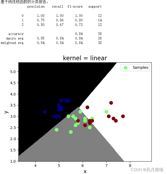
bg = classification_report(y_test, y_test_pred)
print('基于线性核函数的分类报告：', bg, sep ='\n')
#绘制分类边界线
l, r = x[:,0].min() - 1, x[:,0].max() + 1
b, t = x[:,1].min() - 1, x[:,1].max() + 1
n = 500
grid_x,grid_y = np.meshgrid(np.linspace(l,r,n), np.linspace(b,t,n))
bg_x = np.column_stack((grid_x.ravel(), grid_y.ravel()))
bg_y = model.predict(bg_x)
grid_z = bg_y.reshape(grid_x.shape)
#画图显示样本数据
plt.title('kernel = linear', fontsize = 16)
plt.xlabel('x',fontsize = 14)
plt.ylabel('y',fontsize = 14)
plt.tick_params(labelsize = 10)
plt.pcolormesh(grid_x, grid_y, grid_z, cmap = 'gray')
plt.scatter(x_test[:,0], x_test[:,1], s = 80, c = y_test, cmap = 'jet', label = 'Samples')
plt.legend()
plt.show()

【运行结果】

5.1.1 在选择核函数时，一般遵循如下原则：

如果特征非常多或者样本数远少于特征数，数据更偏向线性可分，选择线性核函数效果会更好。
线性和函数的参数少，速度快；径向基核函数的参数多，分类结果非常依赖参数，需要交叉验证或网格搜索最佳参数。
径向基核函数应用最广，对于小样本还是大样本、高纬度还是低纬度等情况都适用。

5.2 波士顿房价

#导人画图工具
import matplotlib.pyplot as plt
#导人波士顿房价数据集
#from sklearn.datasets import load_boston
import pandas as pd
import numpy as np
data_url = "http://lib.stat.cmu.edu/datasets/boston"
raw_df = pd.read_csv(data_url, sep="\s+", skiprows=22, header=None)
data = np.hstack([raw_df.values[::2, :], raw_df.values[1::2, :2]])
target = raw_df.values[1::2, 2]
#打印数据集中的键
print(raw_df.keys())
#导人数据集拆分工具
from sklearn.model_selection import train_test_split
#建立训练集和测试集
X,y=data, target
X_train, X_test, y_train, y_test=train_test_split(X,y,random_state=8)
#导人数据预处理工具
from sklearn.preprocessing import StandardScaler
#对训练集和测试集进行数据预处理
scaler=StandardScaler()
scaler.fit(X_train)
X_train_scaled=scaler.transform(X_train)
X_test_scaled=scaler.transform(X_test)
#将预处理后的数据特征最大值和最小值用散点图表示n
#导人支持向量机回归模型
from sklearn.svm import SVR
#用预处理后的数据重新训练模型
for kernel in ['linear', 'rbf']:
    svr=SVR(kernel=kernel)
    svr.fit(X_train_scaled, y_train)
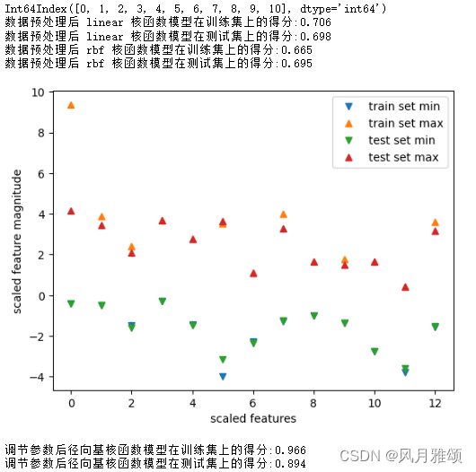
    print('数据预处理后',kernel,'核函数模型在训练集上的得分:{:.3f}'.format(svr.score(X_train_scaled,y_train)))
    print('数据预处理后',kernel,'核函数模型在测试集上的得分:{:.3f}'. format(svr.score(X_test_scaled,y_test)))
plt.plot(X_train_scaled.min(axis=0),'v',label='train set min')
plt.plot(X_train_scaled.max(axis=0),'^', label='train set max')
plt.plot(X_test_scaled.min(axis=0), 'v', label='test set min')
plt.plot(X_test_scaled.max(axis=0), '^', label='test set max')
#设置图注位置为最佳位置
plt.legend(loc='best')
#设置横纵轴标题
plt.xlabel('scaled features')
plt.ylabel('scaled feature magnitude')
plt.show()
#设置径向基核模型的C参数和 gamma参数
svr=SVR(C=100, gamma=0.1)
svr.fit(X_train_scaled, y_train)
print('调节参数后径向基核函数模型在训练集上的得分:{:.3f}'.format(svr.score(X_train_scaled, y_train)))
print('调节参数后径向基核函数模型在测试集上的得分:{:.3f}'.format(svr.score(X_test_scaled, y_test)))

【运行结果】