基于机器学习的假新闻检测 -- 机器学习项目基础篇（14）

不同平台上的假新闻正在广泛传播，这是一个令人严重关切的问题，因为它导致社会稳定和人们之间建立的纽带的永久破裂。很多研究已经开始关注假新闻的分类。
在这里，我们将尝试在Python中的机器学习的帮助下解决这个问题。

主要步骤

• 导入库和数据集
• 数据预处理
• 新闻栏目的预处理与分析
• 将文本转换为矢量
• 模型训练、评估和预测

1. 导入库和数据集

• Pandas：用于导入数据集。
• Seaborn/Matplotlib：用于数据可视化。

import pandas as pd
import seaborn as sns
import matplotlib.pyplot as plt

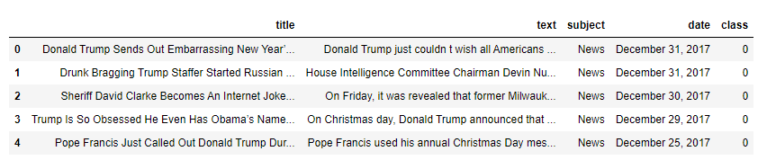
data = pd.read_csv('News.csv',index_col=0)
data.head()

2. 数据预处理

data.shape

输出：

(44919, 5)

由于标题、主题和日期栏对新闻的识别没有帮助。所以，我们可以删除这些列。

data = data.drop(["title", "subject","date"], axis = 1)

现在，我们必须检查是否有任何空值（我们将删除那些行）

data.isnull().sum()

输出：

text     0
class    0 

现在我们必须对数据集进行打乱，以防止模型出现偏差。之后我们将重置索引，然后删除它。因为索引列对我们没有用。

# Shuffling
data = data.sample(frac=1)
data.reset_index(inplace=True)
data.drop(["index"], axis=1, inplace=True)

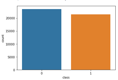
让我们使用下面的代码来探索每个类别中的唯一值。

sns.countplot(data=data,
              x='class',
              order=data['class'].value_counts().index)

3. 新闻栏目的预处理与分析

首先，我们将从文本中删除所有的停用词，标点符号和任何不相关的空格。NLTK库是必需的，它的一些模块需要下载。因此，运行下面的代码。

from tqdm import tqdm
import re
import nltk
nltk.download('punkt')
nltk.download('stopwords')
from nltk.corpus import stopwords
from nltk.tokenize import word_tokenize
from nltk.stem.porter import PorterStemmer
from wordcloud import WordCloud

一旦我们有了所有需要的模块，我们就可以创建一个函数名预处理文本。此函数将预处理作为输入的所有数据。

def preprocess_text(text_data):
    preprocessed_text = []
      
    for sentence in tqdm(text_data):
        sentence = re.sub(r'[^\w\s]', '', sentence)
        preprocessed_text.append(' '.join(token.lower()
                                  for token in str(sentence).split()
                                  if token not in stopwords.words('english')))
  
    return preprocessed_text

要在文本列中的所有新闻中实现该函数，请运行以下命令。

preprocessed_review = preprocess_text(data['text'].values)
data['text'] = preprocessed_review

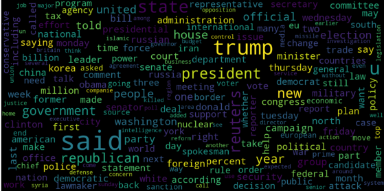
让我们分别为假新闻和真实的新闻可视化WordCloud。

# Real
consolidated = ' '.join(
    word for word in data['text'][data['class'] == 1].astype(str))
wordCloud = WordCloud(width=1600,
                      height=800,
                      random_state=21,
                      max_font_size=110,
                      collocations=False)
plt.figure(figsize=(15, 10))
plt.imshow(wordCloud.generate(consolidated), interpolation='bilinear')
plt.axis('off')
plt.show()

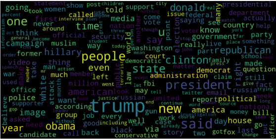
# Fake
consolidated = ' '.join(
    word for word in data['text'][data['class'] == 0].astype(str))
wordCloud = WordCloud(width=1600,
                      height=800,
                      random_state=21,
                      max_font_size=110,
                      collocations=False)
plt.figure(figsize=(15, 10))
plt.imshow(wordCloud.generate(consolidated), interpolation='bilinear')
plt.axis('off')
plt.show()

现在，让我们绘制前20个最常见单词的条形图。

from sklearn.feature_extraction.text import CountVectorizer
  
  
def get_top_n_words(corpus, n=None):
    vec = CountVectorizer().fit(corpus)
    bag_of_words = vec.transform(corpus)
    sum_words = bag_of_words.sum(axis=0)
    words_freq = [(word, sum_words[0, idx])
                  for word, idx in vec.vocabulary_.items()]
    words_freq = sorted(words_freq, key=lambda x: x[1],
                        reverse=True)
    return words_freq[:n]
  
  
common_words = get_top_n_words(data['text'], 20)
df1 = pd.DataFrame(common_words, columns=['Review', 'count'])
  
df1.groupby('Review').sum()['count'].sort_values(ascending=False).plot(
    kind='bar',
    figsize=(10, 6),
    xlabel="Top Words",
    ylabel="Count",
    title="Bar Chart of Top Words Frequency"
)

4. 将文本转换为矢量

在将数据转换为矢量之前，将其分为训练和测试。

from sklearn.model_selection import train_test_split
from sklearn.metrics import accuracy_score
from sklearn.linear_model import LogisticRegression
  
x_train, x_test, y_train, y_test = train_test_split(data['text'], 
                                                    data['class'], 
                                                    test_size=0.25)

现在我们可以使用TfidfVectorizer将训练数据转换为向量。

from sklearn.feature_extraction.text import TfidfVectorizer
  
vectorization = TfidfVectorizer()
x_train = vectorization.fit_transform(x_train)
x_test = vectorization.transform(x_test)

5. 模型训练、评估和预测

现在，数据集已经准备好可以训练模型。
对于训练，我们将使用Logistic回归并使用accuracy_score评估预测准确性。

from sklearn.linear_model import LogisticRegression
  
model = LogisticRegression()
model.fit(x_train, y_train)
  
# testing the model
print(accuracy_score(y_train, model.predict(x_train)))
print(accuracy_score(y_test, model.predict(x_test)))

输出：

0.993766511324171
0.9893143365983972

让我们使用决策树分类器进行训练。

from sklearn.tree import DecisionTreeClassifier
  
model = DecisionTreeClassifier()
model.fit(x_train, y_train)
  
# testing the model
print(accuracy_score(y_train, model.predict(x_train)))
print(accuracy_score(y_test, model.predict(x_test)))

输出：

0.9999703167205913
0.9951914514692787

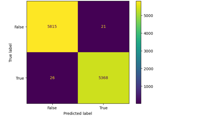
决策树分类器的混淆矩阵可以用下面的代码实现。

# Confusion matrix of Results from Decision Tree classification
from sklearn import metrics
cm = metrics.confusion_matrix(y_test, model.predict(x_test))
  
cm_display = metrics.ConfusionMatrixDisplay(confusion_matrix=cm,
                                            display_labels=[False, True])
  
cm_display.plot()
plt.show()

总结

决策树分类器和Logistic回归表现良好。