复现《Nature communications》图表：ggplot展示多组基因富集结果+显著性区分

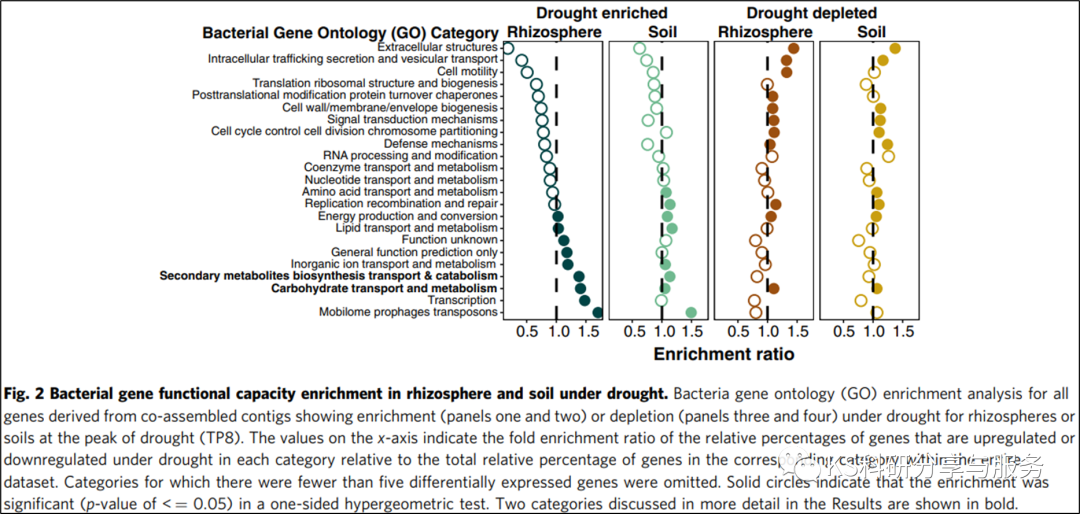
无意中看到NC上一篇文章的富集结果图，觉得挺不错的，也有值得学习的地方，就借鉴一下，复现它。要复现的图片是文章中的Figure2，看出的话其实就是气泡图，类似于之前我们讲过的多组气泡图（复现《nature communications》图表（四）：ggplot画多组富集气泡图）。但是不同之处在于将这4组分开展示了，而且还有一个特点就是实心圆表示显著的，空心圆表示不显著的。万变不离其宗，ggplot就可以实现，来盘它！

因为原文中没有提供数据，所以我自己根据图瞎编了一组数据，没有意义。

A <- read.csv("A.csv",header = T)
library(forcats)
A$Annotation <- as.factor(A$Annotation)
A$Annotation <- fct_inorder(A$Annotation)
library(ggplot2)

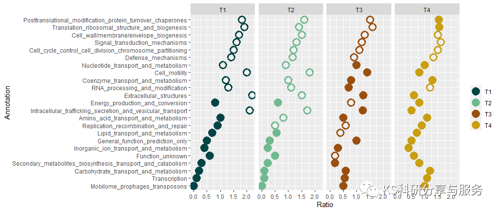
横轴就是Ratio，纵轴是富集terms，这都没问题，然后填充按照分组，并赋予和文章中类似的颜色。然后就是按照分组做四个图，最重要的一步就是在构建数据的时候添加上显著性这一行，然后使用两个geom_point图层实现。

ggplot(A, aes(x=Ratio, y=Annotation,colour=Tissue)) +
  scale_colour_manual(name="",values = c("#004445","#6FB98F","#9B4F0F","#C99E10"))+
  scale_shape_manual(name="",values=c(1,1,19,19))+facet_wrap(~Tissue,ncol=4)+
  geom_point(size = 4,stroke = 2, shape=21)+
  geom_point(data = A[A$sig=='Y',], shape=16,size=5)

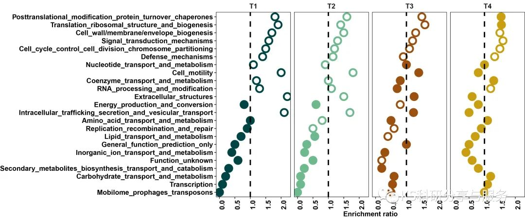
接着添加竖线，更改坐标轴。

ggplot(A, aes(x=Ratio, y=Annotation,colour=Tissue)) +
  scale_colour_manual(name="",values = c("#004445","#6FB98F","#9B4F0F","#C99E10"))+
  scale_shape_manual(name="",values=c(1,1,19,19))+facet_wrap(~Tissue,ncol=4)+
  geom_point(size = 4,stroke = 2, shape=21)+
  geom_point(data = A[A$sig=='Y',], shape=16,size=5)+
  theme_bw()+
  geom_vline(aes(xintercept=1),colour="Black",size=1,linetype="dashed")+
  xlab("Enrichment ratio")

最后修改theme主题，将图片导出保存即可。要完全达到文章中的样子，需要后续在AI中进行修饰。

p <- ggplot(A, aes(x=Ratio, y=Annotation,colour=Tissue)) +
  scale_colour_manual(name="",values = c("#004445","#6FB98F","#9B4F0F","#C99E10"))+
  scale_shape_manual(name="",values=c(1,1,19,19))+facet_wrap(~Tissue,ncol=4)+
  geom_point(size = 4,stroke = 2, shape=21)+
  geom_point(data = A[A$sig=='Y',], shape=16,size=5)+
  theme_bw()+
  geom_vline(aes(xintercept=1),colour="Black",size=1,linetype="dashed")+
  xlab("Enrichment ratio")+
  theme(axis.text.x=element_text(size=11,color="black",face="bold",angle=90), 
        axis.text.y=element_text(size=11,color="black",face="bold"), 
        axis.title=element_text(size=11,face="bold"),text=element_text(size=10))+
  theme(legend.text = element_text(colour="black", size = 11, face = "bold"))+
  theme(legend.position = "none")+
  theme(panel.grid.major = element_blank(),
        panel.grid.minor = element_blank(),
        strip.background = element_blank(),
        panel.border = element_rect(colour = "black")) +
  theme(strip.text = element_text(size=11,face="bold"))+ylab("")

ggsave(filename = "p.pdf",plot = p,width=12,height=5)

还是挺有意思的。想要示例数据的小伙伴，可至我的公众号《KS科研分享与服务》，感谢您的支持！