


在 机器学习入门 — 基于随机森林的气温预测(一)使用随机森林算法完成基本建模任务 中,只用了2016年一个年份的数据来进行实验,本文将增加数据量,把 2011 - 2016 年的数据都拿进来,与原结果进行一个对比
数据展示
# 导入工具包
import pandas as pd
# 读取数据
features = pd.read_csv('data/temps_extended.csv')
features.head()
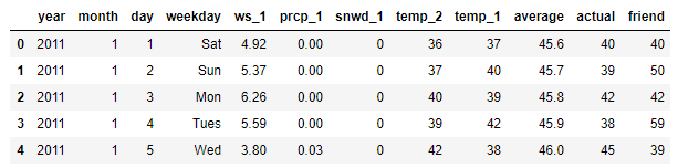
本数据表中:
- year,moth,day,wek分别表示的具体的时间
- ws_1:昨天的风速
- prcp_1: 昨天的降水
- snwd_1:昨天的积雪深度
- temp_ 2:前天的最高温度值
- temp_ 1:昨天的最高温度值
- average: 在历史中,每年这一天的平均最高温度值
- actual: 这就是我们的标签值了,当天的真实最高温度
- friend: 朋友的评价
在此可以到,新的数据集中,数据规模发生了变化,数据量扩充到2191条并且加入了新的天气指标:ws_1、prcp_1、snwd_1
画图看一下新特征
# 设置整体布局
fig, ((ax1, ax2), (ax3, ax4)) = plt.subplots(nrows=2, ncols=2, figsize = (15,10))
fig.autofmt_xdate(rotation = 45)
# 平均最高气温
ax1.plot(dates, features['average'])
ax1.set_xlabel('')
ax1.set_ylabel('Temperature (F)')
ax1.set_title('Historical Avg Max Temp')
# 风速
ax2.plot(dates, features['ws_1'], 'r-')
ax2.set_xlabel('')
ax2.set_ylabel('Wind Speed (mph)')
ax2.set_title('Prior Wind Speed')
# 降水
ax3.plot(dates, features['prcp_1'], 'r-')
ax3.set_xlabel('Date')
ax3.set_ylabel('Precipitation (in)')
ax3.set_title('Prior Precipitation')
# 积雪
ax4.plot(dates, features['snwd_1'], 'ro')
ax4.set_xlabel('Date')
ax4.set_ylabel('Snow Depth (in)')
ax4.set_title('Prior Snow Depth')

plt.tight_layout(pad=2)

上面这个图表中,我们能知道了特征数据的走势
下面我们再按季节做分布,看看 昨天的最高温度值与昨天的降水 这两个特征的用途
# 创建季节变量
seasons = []
# 设定好春夏秋冬
for month in features['month']:
    if month in [1, 2, 12]:
        seasons.append('winter')
    elif month in [3, 4, 5]:
        seasons.append('spring')
    elif month in [6, 7, 8]:
        seasons.append('summer')
    elif month in [9, 10, 11]:
        seasons.append('fall')
# 整合数据
reduced_features = features[['temp_1', 'prcp_1', 'average', 'actual']]
reduced_features['season'] = seasons
reduced_features.head()
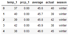
下面使用 Seaborn 画相关矩阵图,来查看多个变量之间的联系
Seaborn其实是在matplotlib的基础上进行了更高级的API封装,从而使得作图更加容易,而且它能高度兼容numpy与pandas数据结构以及scipy与statsmodels等统计模式。
# 导入 seaborn 工具包
import seaborn as sns
sns.set(style="ticks", color_codes=True);
# 定义颜色
palette = sns.xkcd_palette(['dark blue', 'dark green', 'gold', 'orange'])
# 绘制 pairplot
sns.pairplot(reduced_features, hue = 'season', diag_kind = 'kde', palette= palette, plot_kws=dict(alpha = 0.7),
                   diag_kws=dict(shade=True));

通过此矩阵图我们可以看出,temp_1 与 actual 有很强的正比关系
数据预处理
数据的预处理和以前一样
# 导入工具包
import numpy as np
from sklearn.model_selection import train_test_split
# 独热编码处理数据
features = pd.get_dummies(features)
# 设定 features and labels
labels = features['actual']
features = features.drop('actual', axis = 1)
# 将特征转换为列表格式
feature_list = list(features.columns)

features = np.array(features)
labels = np.array(labels)
# 划分数据集
train_features, test_features, train_labels, test_labels = train_test_split(features, labels,
                                                                            test_size = 0.25, random_state = 42)
这里训练效果做一个对比
旧数据集
先看一下旧数据集做出来的结果
# 导入工具包
import pandas as pd
import numpy as np
from sklearn.model_selection import train_test_split
from sklearn.ensemble import RandomForestRegressor
# 读取数据集
original_features = pd.read_csv('data/temps.csv')
# 独热编码处理数据
original_features = pd.get_dummies(original_features)
# 指定标签
original_labels = np.array(original_features['actual'])
# 指定特征集
original_features= original_features.drop('actual', axis = 1)
# 保存特征名称,转化为list格式
original_feature_list = list(original_features.columns)
# 转化为 np.array
original_features = np.array(original_features)
# 划分数据集
original_train_features, original_test_features, original_train_labels, original_test_labels = train_test_split(original_features,
                                                                                                                original_labels,
                                                                                                                test_size = 0.25,
                                                                                                                random_state = 42)
# 建模
rf = RandomForestRegressor(n_estimators= 1000, random_state=42)
# 训练模型
rf.fit(original_train_features, original_train_labels);
# 预测
predictions = rf.predict(original_test_features)
# 算平均绝对误差
errors = abs(predictions - original_test_labels)
# 算平均绝对百分比误差
mape = 100 * (errors / original_test_labels)
accuracy = 100 - np.mean(mape)
# 输出结果
print('Average absolute error:', round(np.mean(errors), 2))
print('Accuracy:', round(accuracy, 2), '%')
Average absolute error: 3.83
Accuracy: 93.99 %
旧数据集扩量
接下来是使用新的数据集,但是只增加数据量,不添加新的特征进来
from sklearn.ensemble import RandomForestRegressor
# 查找原始特征索引
original_feature_indices = [feature_list.index(feature) for feature in
                                      feature_list if feature not in
                                      ['ws_1', 'prcp_1', 'snwd_1']]
# 使用旧数据索引值在新数据中得到训练数据
original_train_features = train_features[:,original_feature_indices]
# 使用旧数据索引值在新数据中得到测试数据
original_test_features = test_features[:, original_feature_indices]
# 建模
rf = RandomForestRegressor(n_estimators= 100, random_state=42)
# 训练
rf.fit(original_train_features, train_labels);
# 预测结果
baseline_predictions = rf.predict(original_test_features)
# 算平均绝对误差
baseline_errors = abs(baseline_predictions - test_labels)
# 算平均绝对百分比误差
baseline_mape = 100 * np.mean((baseline_errors / test_labels))
baseline_accuracy = 100 - baseline_mape
# 打印
print('Average absolute error:', round(np.mean(baseline_errors), 2))
print('Accuracy:', round(baseline_accuracy, 2), '%')
Average absolute error: 3.76
Accuracy: 93.7 %
根据这两个输出结果的对比,说明了数据量增大对结果起到了一定的促进作用
新数据集
# 导入工具包
from sklearn.ensemble import RandomForestRegressor
# 建模
rf_exp = RandomForestRegressor(n_estimators= 100, random_state=42)
# 训练
rf_exp.fit(train_features, train_labels)
# 预测结果
predictions = rf_exp.predict(test_features)
# 算平均绝对误差
errors = abs(predictions - test_labels)
# 算平均绝对百分比误差
mape = np.mean(100 * (errors / test_labels))
accuracy = 100 - mape
# 算平均绝对百分比误差的新旧数据集差值
improvement_baseline = 100 * abs(mape - baseline_mape) / baseline_mape

#打印
print('Improvement over baseline:', round(improvement_baseline, 2), '%')
print('Average absolute error:', round(np.mean(errors), 4))
print('Accuracy:', round(accuracy, 2), '%')
Improvement over baseline: 0.52 %
Average absolute error: 3.7161
Accuracy: 93.73 %
特征重要性
因为在新的数据集中,我们增加了新的特征进来
# 特征名称
importances = list(rf_exp.feature_importances_)
# 拿到特征数据
feature_importances = [(feature, round(importance, 2)) for feature, importance in zip(feature_list, importances)]
# 排序
feature_importances = sorted(feature_importances, key = lambda x: x[1], reverse = True)
# 打印
[print('特征: {:20} 重要性: {}'.format(*pair)) for pair in feature_importances]
特征: temp_1               重要性: 0.83
特征: average              重要性: 0.06
特征: ws_1                 重要性: 0.02
特征: temp_2               重要性: 0.02
特征: friend               重要性: 0.02
特征: year                 重要性: 0.01
特征: month                重要性: 0.01
特征: day                  重要性: 0.01
特征: prcp_1               重要性: 0.01
特征: snwd_1               重要性: 0.0
特征: weekday_Fri          重要性: 0.0
特征: weekday_Mon          重要性: 0.0
特征: weekday_Sat          重要性: 0.0
特征: weekday_Sun          重要性: 0.0
特征: weekday_Thurs        重要性: 0.0
特征: weekday_Tues         重要性: 0.0
特征: weekday_Wed          重要性: 0.0
对特征重要性进行可视化
# 设定绘图风格
plt.style.use('fivethirtyeight')
# 指定位置
x_values = list(range(len(importances)))
# 绘图
plt.bar(x_values, importances, orientation = 'vertical', color = 'r', edgecolor = 'k', linewidth = 1.2)
# 指定名称
plt.xticks(x_values, feature_list, rotation='vertical')
# 绘图
plt.ylabel('Importance')
plt.xlabel('Variable')
plt.title('Variable Importances')

这里我们看到,temp_1 特征最重要,还有一些特征完全不起作用,所以关于在训练中特征,其特征重要性累加后在95%就可以,就是说有多少个特征的特征多样性累加达到95%,使用这些特征就够了
# 对特征重要性排序
sorted_importances = [importance[1] for importance in feature_importances]
sorted_features = [importance[0] for importance in feature_importances]
# 计算累加值,累计重要性
cumulative_importances = np.cumsum(sorted_importances)
# 绘制折线图
plt.plot(x_values, cumulative_importances, 'g-')
# 画一条红虚线 0.95的界限
plt.hlines(y = 0.95, xmin=0, xmax=len(sorted_importances), color = 'r', linestyles = 'dashed')
# X周名称
plt.xticks(x_values, sorted_features, rotation = 'vertical')
# 绘图
plt.xlabel('Variable')
plt.ylabel('Cumulative Importance')
plt.title('Cumulative Importances')

通过这张图表也可以看出,我们前6项特征的和达到了95%
接下来,我们使用这6项特征再次进行训练
# 选择这6项特征
important_feature_names = [feature[0] for feature in feature_importances[0:6]]
# 找到他们的索引
important_indices = [feature_list.index(feature) for feature in important_feature_names]
# 拿到训练集与测试集
important_train_features = train_features[:, important_indices]
important_test_features = test_features[:, important_indices]
# 建模
rf_exp = RandomForestRegressor(n_estimators= 100, random_state=42)
# 训练
rf_exp.fit(important_train_features, train_labels)
# 预测
predictions = rf_exp.predict(important_test_features)
# 算平均绝对误差
errors = abs(predictions - test_labels)
# 算平均绝对百分比误差
mape = 100 * (errors / test_labels)
accuracy = 100 - np.mean(mape)
# 打印
print('Average absolute error:', round(np.mean(errors), 4))
print('Accuracy:', round(accuracy, 2), '%')
Average absolute error: 3.829
Accuracy: 93.56 %
结果来看,效果反而下降了,其实随机森林的算法本身就会考虑特征的问题,会优先选择有价值的,我们认为的去掉一些,相当于可供候选的就少了,也就会出现这样的现象
计算 Trade-Offs
Run-Time
虽然说模型没有提升,反而精度还有一点点的下降,那我们再看看他们在时间效率层面上有没有进步
计算放入所有特征时建模与测试消耗的时间
# 导入包
import time
# 建立空list
all_features_time = []
# 一次不太准,所以算10次取平均
for _ in range(10):
    start_time = time.time()
    rf_exp.fit(train_features, train_labels)
    all_features_predictions = rf_exp.predict(test_features)
    end_time = time.time()
    all_features_time.append(end_time - start_time)
all_features_time = np.mean(all_features_time)
print('使用所有特征时建模与测试的平均消耗时间:', round(all_features_time, 2), '秒')
使用所有特征时建模与测试的平均消耗时间: 0.72 秒
计算放入所有特征时建模与测试消耗的时间
# 导入包
import time
# 建立空list
reduced_features_time = []
# 一次不太准,所以算10次取平均
for _ in range(10):
    start_time = time.time()
    rf_exp.fit(important_train_features, train_labels)
    reduced_features_predictions = rf_exp.predict(important_test_features)
    end_time = time.time()
    reduced_features_time.append(end_time - start_time)
reduced_features_time = np.mean(reduced_features_time)
print('使用所有特征时 建模与测试的平均消耗时间:', round(reduced_features_time, 2), '秒')
使用所有特征时 建模与测试的平均消耗时间: 0.5 秒
我们看到,虽然精度降低了,但是建模与测试消耗的时间减少了0.22秒
Accuracy vs Run-Time
#用预测值来计算评估结果
all_accuracy =  100 * (1- np.mean(abs(all_features_predictions - test_labels) / test_labels))
reduced_accuracy = 100 * (1- np.mean(abs(reduced_features_predictions - test_labels) / test_labels))
# 创建df来存结果
comparison = pd.DataFrame({'features': ['all (17)', 'reduced (5)'],
                           'run_time': [round(all_features_time, 2), round(reduced_features_time, 2)],
                           'accuracy': [round(all_accuracy, 2), round(reduced_accuracy, 2)]})
comparison[['features', 'accuracy', 'run_time']]
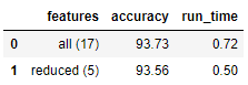
relative_accuracy_decrease = 100 * (all_accuracy - reduced_accuracy) / all_accuracy
print('相对准确率下降:', round(relative_accuracy_decrease, 3), '%')
relative_runtime_decrease = 100 * (all_features_time - reduced_features_time) / all_features_time
print('相对时间效率下降:', round(relative_runtime_decrease, 3), '%')
相对准确率下降: 0.187 %
相对时间效率下降: 30.792 %
这两种结果展示,可以看到准确率并没有太大的差别,下降了0.187 %,但是运行时间差别还是比较大的,下降了30.792 %,所以实际中我们也得综合来考虑下性能问题
总结
对只有一年的数据量的数据集、完整的新数据集、按照95%阈值选择的部分重要特征的数据集进行比较
# 导入包
import pandas as pd
import numpy as np
from sklearn.model_selection import train_test_split
# 读入旧数据
original_features = pd.read_csv('data/temps.csv')
# 独热编码处理数据
original_features = pd.get_dummies(original_features)
# 指定标签
original_labels = np.array(original_features['actual'])
# 特征集
original_features= original_features.drop('actual', axis = 1)
# 获取特征列表
original_feature_list = list(original_features.columns)
# 转换成np.array形式
original_features = np.array(original_features)
# 数据集划分
original_train_features, original_test_features, original_train_labels, original_test_labels = train_test_split(original_features,
original_labels,
test_size = 0.25,
random_state = 42)
# 拿到旧数据集的特征索引
original_feature_indices = [feature_list.index(feature) for feature in
feature_list if feature not in
['ws_1', 'prcp_1', 'snwd_1']]
# 创建旧数据集的特征的测试集
original_test_features = test_features[:, original_feature_indices]
# 设定空list
original_features_time = []
# 训练和测试 循环10次
for _ in range(10):
start_time = time.time()
rf.fit(original_train_features, original_train_labels)
original_features_predictions = rf.predict(original_test_features)
end_time = time.time()
original_features_time.append(end_time - start_time)
# 计算平均时间
original_features_time = np.mean(original_features_time)
# 计算MAE
original_mae = np.mean(abs(original_features_predictions - test_labels))
exp_all_mae = np.mean(abs(all_features_predictions - test_labels))
exp_reduced_mae = np.mean(abs(reduced_features_predictions - test_labels))
# 计算旧数据的accuracy
original_accuracy = 100 * (1 - np.mean(abs(original_features_predictions - test_labels) / test_labels))
# 创建df来存结果
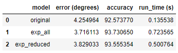
model_comparison = pd.DataFrame({'model': ['original', 'exp_all', 'exp_reduced'],
'error (degrees)': [original_mae, exp_all_mae, exp_reduced_mae],
'accuracy': [original_accuracy, all_accuracy, reduced_accuracy],
'run_time (s)': [original_features_time, all_features_time, reduced_features_time]})
model_comparison = model_comparison[['model', 'error (degrees)', 'accuracy', 'run_time (s)']]
# 最后做绘图总结
# 设置总体布局
fig, (ax1, ax2, ax3) = plt.subplots(nrows=3, ncols=1, figsize = (8,16), sharex = True)
# X轴名称定义
x_values = [0, 1, 2]
labels = list(model_comparison['model'])
plt.xticks(x_values, labels)
# 定义字体大小
fontdict = {'fontsize': 18}
fontdict_yaxis = {'fontsize': 14}
# 比较 Error
ax1.bar(x_values, model_comparison['error (degrees)'], color = ['b', 'r', 'g'], edgecolor = 'k', linewidth = 1.5)
ax1.set_ylim(bottom = 3.5, top = 4.5)
ax1.set_ylabel('Error (degrees) (F)', fontdict = fontdict_yaxis)
ax1.set_title('Model Error Comparison', fontdict= fontdict)
# 比较 Accuracy
ax2.bar(x_values, model_comparison['accuracy'], color = ['b', 'r', 'g'], edgecolor = 'k', linewidth = 1.5)
ax2.set_ylim(bottom = 92, top = 94)
ax2.set_ylabel('Accuracy (%)', fontdict = fontdict_yaxis)
ax2.set_title('Model Accuracy Comparison', fontdict= fontdict)
# 比较 Run Time
ax3.bar(x_values, model_comparison['run_time (s)'], color = ['b', 'r', 'g'], edgecolor = 'k', linewidth = 1.5)
ax3.set_ylim(bottom = 0, top = 1)
ax3.set_ylabel('Run Time (sec)', fontdict = fontdict_yaxis)
ax3.set_title('Model Run-Time Comparison', fontdict= fontdict)

original 代表旧数据,就是只有一年的数据量的数据集
exp_all 代表完整的新数据集
exp_reduced 代表按照95%阈值选择的部分重要特征的数据集
结果比较明显,数据量和特征越多,效果也会越好,但是时间效率也会降低


 576
576


 被折叠的 条评论
为什么被折叠?
被折叠的 条评论
为什么被折叠?
 到【灌水乐园】发言


