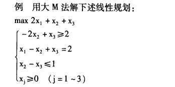
大M法的python编程求解和python包求解

最新推荐文章于 2020-04-26 20:26:26 发布

w²大大

最新推荐文章于 2020-04-26 20:26:26 发布

阅读量1.7k

点赞数 3

分类专栏： python学习文章标签： python 机器学习算法线性规划

本文链接：https://blog.csdn.net/qq_42585108/article/details/105612305

版权

python学习专栏收录该内容

76 篇文章 16 订阅

订阅专栏

大M法的python编程求解和python包求解

一、大M算法的求解步骤讲解

单纯形法的步骤是从一个初始极点出发，不断找到更优的相邻极点，直到找到最优的极点（或极线）。
消去xBxB x_BxB得到问题的字典表达，即：
mincTBB−1b+(cTN−cTBB−1N)xNmin⁡cBTB−1b+(cNT−cBTB−1N)xN \min c^T_BB{-1}b+(c^T_N-cT_BB^{-1}N)x_NmincBTB−1b+(cNT−cBTB−1N)xN
s.t. B−1b−B−1NxN≥0B−1b−B−1NxN≥0 B^{-1}b-B{-1}Nx_N\ge 0B−1b−B−1NxN≥0
xN≥0xN≥0 x_N\ge 0xN≥0
称(cTN−cTBB−1N)i(cNT−cBTB−1N)i (c^T_N-cT_BB^{-1}N)_i(cNT−cBTB−1N)i为第ii ii个非基变量的残差(reduced cost)，如果残差小于0，那么说明这个非基变量还没有满足最优条件。直观上来看，这个非基变量取稍稍大于0的数就可以继续优化目标函数了。我们选择一个基变量和这个非基变量对换，就可以找到更优的相邻极点。
另一种理解方法：残差对应的是对偶问题可行条件，小于0表示对偶问题还不可行，需要继续探索。
接下来的问题是具体选择哪个基变量和哪个非基变量进行对换。我们用启发式原则，每次将负数残差(cTN−cTBB−1N)i(cNT−cBTB−1N)i (c^T_N-cT_BB^{-1}N)_i(cNT−cBTB−1N)i最小（绝对值最大）的非基变量xixi x_ixi替换为基变量，同时将(B−1b(B−1N)i)j(B−1b(B−1N)i)j (\frac{B^{-1}b}{(B{-1}N)_i})j((B−1N)iB−1b)j最小值对应的基变量xjxj x_jxj替换为非基变量。这个进基/出基的过程称为pivoting。
另一种表达方式是：minz=cxmin⁡z=cx \min z = cxminz=cx，s.t.Ax=bAx=b Ax = bAx=b的pivoting是每次找出c中最小数对应的非基变量xixi x_ixi，再找出bi/Aijbi/Aij b_i/A{ij}bi/Aij最小的基变量xjxj x_jxj进行对换。
如果是max问题，令c′=−cc′=−c c’=-cc′=−c即可转化为min问题，相对应的，每次pivoting是找出c′c′ c’c′最大值对应的非基变量。

求解例子如图：
在这里插入图片描述

二、python编程求解

# encoding=utf-8
import numpy as np  # python 矩阵操作lib
class Simplex():

    def __init__(self):
        self._A = ""  # 系数矩阵
        self._b = ""  #数组
        self._c = ''  # 约束
        self._B = ''  # 基变量的下标集合
        self.row = 0  # 约束个数

    def solve(self):
        # 读取文件内容，文件结构前两行分别为 变量数 和 约束条件个数
        # 接下来是系数矩阵
        # 然后是b数组
        # 然后是约束条件c
        # 假设线性规划形式是标准形式（都是等式）

        A = []
        b = []
        c = []

        self._A = np.array(A, dtype=float)
        self._b = np.array(b, dtype=float)
        self._c = np.array(c, dtype=float)
        self._A = np.array([[0,2,-1],[0,1,-1]],dtype=float)
        self._b = np.array([-2,1],dtype=float)
        self._A = np.array([[1,-1,1]])# 等式约束系数self._A，3x1维列向量
        self._b = np.array([2])# 等式约束系数self._b，1x1数值
        
        self._c = np.array([2,1,1],dtype=float)
        self._B = []
        self.row = len(self._b)
        self.var = len(self._c)
        (x, obj) = self.Simplex(self._A, self._b, self._c)
        self.pprint(x, obj, A)

    def pprint(self, x, obj, A):
        px = ['x_%d = %f' % (i + 1, x[i]) for i in range(len(x))]
        print(','.join(px))

        print('objective value is : %f' % obj)
        print('------------------------------')
        for i in range(len(A)):
            print('%d-th line constraint value is : %f' % (i + 1, x.dot(A[i])))

    def InitializeSimplex(self, A, b):

        b_min, min_pos = (np.min(b), np.argmin(b))  # 得到最小bi

        # 将bi全部转化成正数
        if (b_min < 0):
            for i in range(self.row):
                if i != min_pos:
                    A[i] = A[i] - A[min_pos]
                    b[i] = b[i] - b[min_pos]
            A[min_pos] = A[min_pos] * -1
            b[min_pos] = b[min_pos] * -1

        # 添加松弛变量
        slacks = np.eye(self.row)
        A = np.concatenate((A, slacks), axis=1)
        c = np.concatenate((np.zeros(self.var), np.ones(self.row)), axis=0)
        # 松弛变量全部加入基,初始解为b
        new_B = [i + self.var for i in range(self.row)]

        # 辅助方程的目标函数值
        obj = np.sum(b)

        c = c[new_B].reshape(1, -1).dot(A) - c
        c = c[0]
        # entering basis
        e = np.argmax(c)

        while c[e] > 0:
            theta = []
            for i in range(len(b)):
                if A[i][e] > 0:
                    theta.append(b[i] / A[i][e])
                else:
                    theta.append(float("inf"))

            l = np.argmin(np.array(theta))

            if theta[l] == float('inf'):
                print('unbounded')
                return False

            (new_B, A, b, c, obj) = self._PIVOT(new_B, A, b, c, obj, l, e)

            e = np.argmax(c)

        # 如果此时人工变量仍在基中，用原变量去替换之
        for mb in new_B:
            if mb >= self.var:
                row = mb - self.var
                i = 0
                while A[row][i] == 0 and i < self.var:
                    i += 1
                (new_B, A, b, c, obj) = self._PIVOT(new_B, A, b, c, obj, new_B.index(mb), i)

        return (new_B, A[:, 0:self.var], b)

    # 算法入口
    def Simplex(self, A, b, c):
        B = ''
        (B, A, b) = self.InitializeSimplex(A, b)

        # 函数目标值
        obj = np.dot(c[B], b)

        c = np.dot(c[B].reshape(1, -1), A) - c
        c = c[0]

        # entering basis
        e = np.argmax(c)
        # 找到最大的检验数，如果大于0，则目标函数可以优化
        while c[e] > 0:
            theta = []
            for i in range(len(b)):
                if A[i][e] > 0:
                    theta.append(b[i] / A[i][e])
                else:
                    theta.append(float("inf"))

            l = np.argmin(np.array(theta))

            if theta[l] == float('inf'):
                print("unbounded")
                return False

            (B, A, b, c, obj) = self._PIVOT(B, A, b, c, obj, l, e)

            e = np.argmax(c)

        x = self._CalculateX(B, A, b, c)
        return (x, obj)

    # 得到完整解
    def _CalculateX(self, B, A, b, c):

        x = np.zeros(self.var, dtype=float)
        x[B] = b
        return x

    # 基变换
    def _PIVOT(self, B, A, b, c, z, l, e):
        # main element is a_le
        # l represents leaving basis
        # e represents entering basis

        main_elem = A[l][e]
        # scaling the l-th line
        A[l] = A[l] / main_elem
        b[l] = b[l] / main_elem

        # change e-th column to unit array
        for i in range(self.row):
            if i != l:
                b[i] = b[i] - A[i][e] * b[l]
                A[i] = A[i] - A[i][e] * A[l]

        # update objective value
        z -= b[l] * c[e]

        c = c - c[e] * A[l]

        # change the basis
        B[l] = e

        return (B, A, b, c, z)


s = Simplex()
s.solve()

x_1 = 0.000000,x_2 = 0.000000,x_3 = 2.000000
objective value is : 2.000000
------------------------------

三、利用python包scipy的优化包optimize

import numpy as np
from scipy import optimize as op

# 给出变量取值范围
x1=(0,None)
x2=(0,None)
x3=(0,None)

#定义给出变量，确定c,A_ub,B_ub,A_eq,B_eq
c = np.array([2,1,1])# 目标函数系数,3x1列向量
A_ub = np.array([[0,2,-1],[0,1,-1]]) # 不等式约束系数A，2x3维矩阵
B_ub = np.array([-2,1])# 等式约束系数B, 2x1维列向量
A_eq = np.array([[1,-1,1]])# 等式约束系数Aeq，3x1维列向量
B_eq = np.array([2])# 等式约束系数beq，1x1数值

#调用函数求解
res=op.linprog(c,A_ub,B_ub,A_eq,B_eq,bounds=(x1,x2,x3))#调用函数进行求解
print(res)

     con: array([3.41133788e-11])
     fun: 1.9999999999762483
 message: 'Optimization terminated successfully.'
     nit: 4
   slack: array([-3.94371202e-11,  3.00000000e+00])
  status: 0
 success: True
       x: array([2.85788627e-13, 5.03802074e-12, 2.00000000e+00])

四、用excel求解

①根据公式自行推导
结果如下：
在这里插入图片描述
②根据excel的自带规划求解
结果如下：

五、分析结果

用四种方式都都能很好的计算出最优解，但在用python包scipy的优化包optimize计算时，发现结果不太一样，百度后仔细一看，原来是精确度的问题。最后求出的目标函数最大值都是2。这四种方式相比之下，发现用python求解是简单，最方便的，而用excel求解太繁琐了，一不小心就要出错，要十分仔细。

参考链接：https://ismango.blog.csdn.net/article/details/105604577

w²大大

关注

3
点赞
踩
7

收藏

觉得还不错? 一键收藏
1
评论
大M法的python编程求解和python包求解

大M法的python编程求解和python包求解一、大M算法的求解步骤讲解二、python编程求解三、利用python包scipy的优化包optimize四、用excel求解五、分析结果一、大M算法的求解步骤讲解单纯形法的步骤是从一个初始极点出发，不断找到更优的相邻极点，直到找到最优的极点（或极线）。消去xBxB x_BxB得到问题的字典表达，即：mincTBB−1b+(cTN...
复制链接

扫一扫