


 超级会员免费看
基于 cPINN 的界面方程求解:原理、实现与结果分析(附Pytorch完整代码)
在科学计算领域,求解偏微分方程(PDEs)一直是一个核心问题。近年来,物理信息神经网络(PINNs)及其变体为解决此类问题提供了新的途径。本文将详细介绍如何利用守恒物理信息神经网络(cPINN)求解特定的界面问题,并结合 Pytorch 代码实现深入探讨其原理与应用。

一、cPINN 方法基础
cPINN 是在离散域上针对非线性守恒定律提出的一种创新方法,它对传统的 PINN 进行了扩展。其核心思想是将计算域划分为多个非重叠的子域,在每个子域上应用 PINN,并通过在相邻子域的公共界面上强制通量等守恒量的连续性来保证整体的守恒性质。

与传统数值方法(如有限元法和有限差分法)不同,PINN 及其变体通过自动微分来近似控制方程中的微分算子,从而避免了对 PDE 的直接离散化,提供了一种无网格算法。然而,PINN 存在一些局限性,例如在处理高维非凸优化问题时可能陷入局部最小值,导致解的精度受限,并且训练成本较高。cPINN 通过域分解有效地解决了这些问题,在每个子域中可以根据解的特性灵活选择网络结构和超参数,如深度、宽度、激活函数、优化算法等,从而降低了优化问题的复杂度,提高了求解精度和效率。
二、问题描述与数学模型
考虑以下扩散问题,其控制方程为:
−
∇
⋅
D
(
x
,
y
)
∇
ϕ
(
x
,
y
)
=
Q
(
x
,
y
)
-\nabla \cdot D(x, y) \nabla \phi(x, y)=Q(x, y)
−∇⋅D(x,y)∇ϕ(x,y)=Q(x,y)
其中, ϕ \phi ϕ 表示中子标通量密度, D ( x , y ) D(x, y) D(x,y) 表示扩散系数, Q ( x , y ) Q(x, y) Q(x,y) 表示外源项。
本算例所用物性参数定义如下:
D ( x , y ) = { D 1 = 4 , if ( x , y ) ∈ [ 0 , 2 3 ] × [ 0 , 1 ] D 2 = 1 , otherwise Q ( x , y ) = { 20 π 2 sin ( π x ) sin ( 2 π y ) , if ( x , y ) ∈ [ 0 , 2 3 ] × [ 0 , 1 ] 20 π 2 sin ( 4 π x ) sin ( 2 π y ) , otherwise \begin{aligned} & D(x, y)= \begin{cases}D_1=4, & \text { if }(x, y) \in\left[0, \frac{2}{3}\right] \times[0,1] \\ D_2=1, & \text { otherwise }\end{cases} \\ & Q(x, y)= \begin{cases}20 \pi^2 \sin (\pi x) \sin (2 \pi y), & \text { if }(x, y) \in\left[0, \frac{2}{3}\right] \times[0,1] \\ 20 \pi^2 \sin (4 \pi x) \sin (2 \pi y), & \text { otherwise }\end{cases} \end{aligned} D(x,y)={D1=4,D2=1, if (x,y)∈[0,32]×[0,1] otherwise Q(x,y)={20π2sin(πx)sin(2πy),20π2sin(4πx)sin(2πy), if (x,y)∈[0,32]×[0,1] otherwise
边界条件为全零边界:
ϕ ( x , y ) = 0 , ∀ ( x , y ) ∈ ∂ Ω \phi(x, y)=0, \quad \forall(x, y) \in \partial \Omega ϕ(x,y)=0,∀(x,y)∈∂Ω
本算例解析解为:
ϕ ( x , y ) = { sin ( π x ) sin ( 2 π y ) , if ( x , y ) ∈ [ 0 , 2 3 ] × [ 0 , 1 ] sin ( 4 π x ) sin ( 2 π y ) , otherwise \phi(x, y)= \begin{cases}\sin (\pi x) \sin (2 \pi y), & \text { if }(x, y) \in\left[0, \frac{2}{3}\right] \times[0,1] \\ \sin (4 \pi x) \sin (2 \pi y), & \text { otherwise }\end{cases} ϕ(x,y)={sin(πx)sin(2πy),sin(4πx)sin(2πy), if (x,y)∈[0,32]×[0,1] otherwise
三、代码实现详解
(一)模型定义
- 网络架构
定义了一个名为PINN的神经网络类,它继承自nn.Module。网络结构由多个全连接层组成,中间层使用Tanh作为激活函数。在__init__方法中,通过循环创建线性层和激活函数层,并将它们组合成一个Sequential模型。同时,使用initialize_weights_glorot_uniform方法对线性层的权重进行初始化,采用 Xavier 均匀分布初始化权重,偏置初始化为 0,这有助于提高网络的训练效果。
class PINN(nn.Module):
    def __init__(self, layers):
        super(PINN, self).__init__()
        self.layers = []
        for i in range(len(layers) - 1):
            self.layers.append(torch.nn.Linear(layers[i], layers[i + 1]))
            if i < len(layers) - 2:
                self.layers.append(torch.nn.Tanh())
        self.net = torch.nn.Sequential(*self.layers)
        self.initialize_weights_glorot_uniform()

    def forward(self, x, y):
        inputs = torch.cat([x, y], dim=1)
        output = self.net(inputs)
        x = inputs[:, 0:1]
        y = inputs[:, 1:2]
        output = output * (x - 1) * (x) * (y - 1) * (y)
        return output

    def initialize_weights_glorot_uniform(self):
        for layer in self.layers:
            if isinstance(layer, torch.nn.Linear):
                init.xavier_uniform_(layer.weight)
                init.constant_(layer.bias, 0.0)
- 物性参数与控制方程残差
定义了diffusion_coefficient和source_term函数来分别计算扩散系数 (D(x,y)) 和源项 (Q(x,y))。在loss_fn函数中,首先通过网络预测得到 (\phi_{pred}),然后计算其关于 (x) 和 (y) 的一阶和二阶导数,最后根据控制方程计算残差,并返回残差的平方的平均值。
def diffusion_coefficient(x, y):
    """D(x, y)"""
    condition = (x <= 2 / 3) & (x >= 0) & (y >= 0) & (y <= 1)
    return torch.where(condition, 4.0, 1.0)


def source_term(x, y):
    """Q(x, y)"""
    condition = (x <= 2 / 3) & (x >= 0) & (y >= 0) & (y <= 1)
    return torch.where(condition, 20 * (torch.pi ** 2) * torch.sin(torch.pi * x) * torch.sin(2 * torch.pi * y),
                       20 * (torch.pi ** 2) * torch.sin(4 * torch.pi * x) * torch.sin(2 * torch.pi * y))


def loss_fn(pinn, x, y):
    # 网络预测
    phi_pred = pinn(x, y)
    D = diffusion_coefficient(x, y)
    Q = source_term(x, y)

    # 梯度计算
    phi_x = torch.autograd.grad(phi_pred, x, grad_outputs=torch.ones_like(phi_pred), create_graph=True)[0]
    phi_y = torch.autograd.grad(phi_pred, y, grad_outputs=torch.ones_like(phi_pred), create_graph=True)[0]

    # 二阶梯度
    phi_xx = torch.autograd.grad(phi_x, x, grad_outputs=torch.ones_like(phi_x), create_graph=True)[0]
    phi_yy = torch.autograd.grad(phi_y, y, grad_outputs=torch.ones_like(phi_y), create_graph=True)[0]

    # 控制方程残差
    residual = -D * (phi_xx + phi_yy) - Q
    return torch.mean(residual ** 2)
- 边界与界面损失
boundary_loss函数用于计算边界条件损失,它通过将边界数据输入网络得到边界上的预测值 ϕ b o u n d a r y \phi_{boundary} ϕboundary,并返回其平方的平均值。interface_loss函数用于计算两个子域在界面处的匹配损失,它接受两个子域的网络模型以及界面数据,计算界面上两个网络预测值的差的平方的平均值。
def boundary_loss(pinn, x_boundary, y_boundary):
    phi_boundary = pinn(x_boundary, y_boundary)
    return torch.mean(phi_boundary ** 2)


def interface_loss(pinn1, pinn2, x_interface, y_interface):
    phi1 = pinn1(x_interface, y_interface)
    phi2 = pinn2(x_interface, y_interface)
    return torch.mean((phi1 - phi2) ** 2)
(二)训练过程
- 数据准备
首先设置了随机种子以确保结果的可复现性。然后定义了网络结构和训练参数,如训练的轮数epochs、不同损失项的权重Wf、Wb、Wi等。接着创建了两个PINN模型实例pinn_left和pinn_right,分别用于左右子域,并将它们迁移到指定的设备(如 GPU 或 CPU)上。同时,还加载了预训练的模型权重。
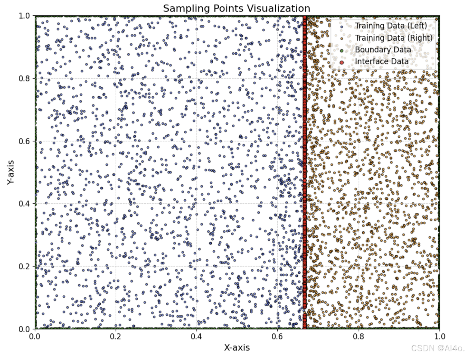
之后,生成了训练数据、边界数据和界面数据。训练数据在左右子域内随机分布,边界数据覆盖了问题的边界条件,界面数据位于两个子域的交界处。这些数据都被转换为可求导的张量,并迁移到指定设备上。
# 设置种子以确保结果可复现
torch.manual_seed(42)

# 定义网络结构
layers = [2] + [100] * 5 + [1]
epochs = 200000
Wf = 1
Wb = 100
Wi = 100

# 创建并迁移模型到指定设备
pinn_left = PINN(layers).to(device)
pinn_right = PINN(layers).to(device)
pinn_left = load_model(pinn_left, "./cPINN/model_Tanh/best_pinn_left.pth")
pinn_right = load_model(pinn_right, "./cPINN/model_Tanh/best_pinn_right.pth")

# 优化器
optimizer = optim.Adam(list(pinn_left.parameters()) + list(pinn_right.parameters()), lr=1e-4)
# 学习率调度器
scheduler = lr_scheduler.ExponentialLR(optimizer, gamma=(1e-7 / 1e-4) ** (1 / epochs))  # 指数衰减学习率

num_f = 2000
num_fe = 200
num_b = 300
num_i = 500

# 训练数据
x_left = torch.cat([torch.rand(num_f, 1) * 2 / 3, torch.rand(num_fe, 1) * 2 / 3 * 0.1 + 2 / 3 * 0.9], dim=0).to(device).requires_grad_()
y_left = torch.cat([torch.rand(num_f, 1), torch.rand(num_fe, 1)], dim=0).to(device).requires_grad_()
x_right = torch.cat([torch.rand(num_f, 1) * (1 - 2 / 3) + 2 / 3, torch.rand(num_fe, 1) * (1 - 2 / 3) * 0.1 + 2 / 3], dim=0).to(device).requires_grad_()
y_right = torch.cat([torch.rand(num_f, 1), torch.rand(num_fe, 1)], dim=0).to(device).requires_grad_()

# 边界数据
x_boundary = torch.cat([torch.zeros(num_b, 1), torch.rand(num_b, 1) * 2 / 3, torch.rand(num_b, 1) * 2 / 3, torch.ones(num_b, 1),
                        torch.rand(num_b, 1) * (1 - 2 / 3) + 2 / 3, torch.rand(num_b, 1) * (1 - 2 / 3) + 2 / 3], dim=0).to(device).requires_grad_()
y_boundary = torch.cat([torch.rand(num_b, 1), torch.ones(num_b, 1), torch.zeros(num_b, 1), torch.rand(num_b, 1),
                        torch.zeros(num_b, 1), torch.ones(num_b, 1)], dim=0).to(device).requires_grad_()
x_boundary_left = torch.cat([torch.zeros(num_b, 1), torch.rand(num_b, 1) * 2 / 3, torch.rand(num_b, 1) * 2 / 3], dim=0).to(device).requires_grad_()
y_boundary_left = torch.cat([torch.rand(num_b, 1), torch.ones(num_b, 1), torch.zeros(numb, 1)], dim=0).to(device).requires_grad_()
x_boundary_right = torch.cat([torch.ones(num_b, 1), torch.rand(num_b, 1) * (1 - 2 / 3) + 2 / 3,
                              torch.rand(num_b, 1) * (1 - 2 / 3) + 2 / 3], dim=0).to(device).requires_grad_()
y_boundary_right = torch.cat([torch.rand(num_b, 1), torch.zeros(num_b, 1), torch.ones(num_b, 1)], dim=0).to(device).requires_grad_()

# 界面数据
x_interface = torch.full((num_i, 1), 2 / 3, requires_grad=True).to(device)
y_interface = torch.rand(num_i, 1, requires_grad=True).to(device)
- 训练循环
在训练循环中,首先将优化器的梯度清零。然后分别计算左右子域的控制方程残差损失loss_left和loss_right,并将它们相加得到loss_f。接着计算边界条件损失loss_b和界面匹配损失loss_i。最后,根据设定的权重计算总损失total_loss,并进行反向传播和优化器更新。同时,使用学习率调度器按照指数衰减的方式调整学习率。
在每一轮训练中,还记录了各种损失值到loss_history字典中,并定期打印训练信息和保存模型。如果当前总损失小于之前记录的最佳损失,则更新最佳损失和最佳模型。
# 初始化损失历史字典
loss_history = {
    'f_loss': [],
    'b_loss': [],
    'i_loss': [],
    'total_loss': []
}
best_loss = float('inf')
best_model_left = None
best_model_right = None

# 检查保存路径是否存在,不存在则创建
model_dir = 'cPINN/model_Tanh'
if not os.path.exists(model_dir):
    os.makedirs(model_dir)

# 训练过程
for epoch in tqdm(range(epochs), desc="Training Epochs"):
    optimizer.zero_grad()

    # 左子区域和右子区域损失
    loss_left = loss_fn(pinn_left, x_left, y_left)
    loss_right = loss_fn(pinn_right, x_right, y_right)

    loss_f = loss_left + loss_right
    # 边界条件损失
    loss_b = boundary_loss(pinn_left, x_boundary_left, y_boundary_left) + boundary_loss(pinn_right, x_boundary_right, y_boundary_right)

    # 界面匹配损失
    loss_i = interface_loss(pinn_left, pinn_right, x_interface, y_interface)

    # 总损失
    total_loss = Wf * loss_f + Wb * loss_b + Wi * loss_i

    total_loss.backward(retain_graph=True)  # 保留计算图
    optimizer.step()
    scheduler.step()  # 更新学习率

    # 记录损失
    loss_history['f_loss'].append(loss_f.item())
    loss_history['b_loss'].append(loss_b.item())
    loss_history['i_loss'].append(loss_i.item())
    loss_history['total_loss'].append(total_loss.item())

    if epoch % 100 == 0:
        print(f"Epoch [{epoch + 1}/{epochs}], F Loss: {loss_f.item():.6f}, B Loss: {loss_b.item():.6f}, I Loss: {loss_i.item():.6f}, Total Loss: {total_loss.item():.6f}")
        print(f'Epoch [{epoch + 1}/{epochs}], Current Learning Rate: {scheduler.get_last_lr()[0]}')
    # 每 10000 次训练保存模型
    if epoch % 10000 == 0:
        # 保存当前模型
        torch.save(pinn_left.state_dict(), f'cPINN/model_Tanh/pinn_left_epoch_{epoch}.pth')
        torch.save(pinn_right.state_dict(), f'cPINN/model_Tanh/pinn_right_epoch_{epoch}.pth')

    # 保存最佳模型(总损失最小)
    if total_loss.item() < best_loss:
        best_loss = total_loss.item()
        best_model_left = pinn_left.state_dict()
        best_model_right = pinn_right.state_dict()

# 保存最佳模型
torch.save(best_model_left, 'cPINN/model_Tanh/best_pinn_left.pth')
torch.save(best_model_right, 'cPINN/model_Tanh/best_pinn_right.pth')
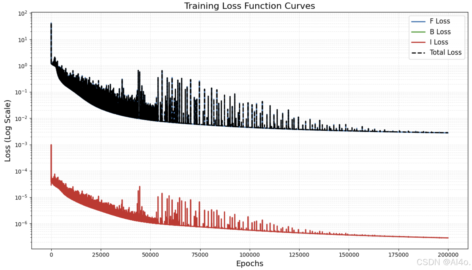
- 损失函数绘制
训练完成后,使用matplotlib库绘制损失函数曲线。包括控制方程残差损失f_loss、边界条件损失b_loss、界面匹配损失i_loss和总损失total_loss。设置了坐标轴标签、标题、对数刻度、图例和网格线,并将图像保存为高分辨率的文件。
# 训练完成后绘制损失函数
epochs_range = range(epochs)

plt.figure(figsize=(12, 7))

# 绘制每个损失函数,优化颜色与线型
plt.plot(epochs_range, loss_history['f_loss'], label='F Loss', color='#1f77b4', linewidth=2)
plt.plot(epochs_range, loss_history['b_loss'], label='B Loss', color='#2ca02c', linewidth=2)
plt.plot(epochs_range, loss_history['i_loss'], label='I Loss', color='#d62728', linewidth=2)
plt.plot(epochs_range, loss_history['total_loss'], label='Total Loss', color='#000000', linestyle='--', linewidth=2)

# 设置坐标轴标签和标题
plt.xlabel('Epochs', fontsize=14)
plt.ylabel('Loss (Log Scale)', fontsize=14)
plt.title('Training Loss Function Curves', fontsize=16)

# 设置对数刻度
plt.yscale('log')

# 增加图例
plt.legend(fontsize=12, loc='upper right')

# 设置网格线,使其不干扰显示
plt.grid(True, which="both", linestyle='--', linewidth=0.7, alpha=0.3)

# 调整布局使其更加紧凑
plt.tight_layout()

# 保存损失图像,设置更高的分辨率
plt.savefig('cPINN/loss_curve.png', dpi=300)

# 显示图像
plt.show()
四、结果评估与可视化
(一)误差计算与分析
在完成模型训练后,计算预测解与解析解之间的误差。通过在测试数据上进行预测,并将预测结果与精确的解析解进行对比,得到绝对误差、相对误差和均方误差。
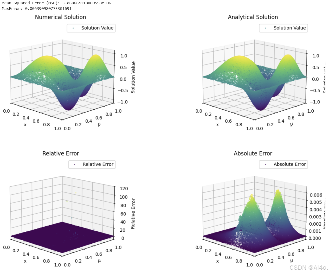
从计算结果来看,绝对误差、相对误差和均方误差在一定程度上反映了模型的预测精度。通过对比预测结果和解析解的可视化图像,可以直观地看出模型在不同区域的预测准确性。在大部分区域,预测结果与解析解的形状和趋势较为吻合。
五、研究总结与展望
在本次研究中,基于 cPINN 方法成功地对简单界面问题进行了求解。通过合理设计网络架构、定义损失函数以及精心准备训练数据,实现了对二维扩散方程的有效逼近。
从结果来看,模型在经过大量的训练后,能够在一定程度上准确地预测分布,并且通过损失函数的下降趋势和误差分析可以验证模型的学习效果。然而,仍然存在一些可以改进的地方。
在未来的研究中,可以考虑进一步优化网络结构,例如尝试不同的层数、神经元数量以及激活函数组合,以寻找更适合该问题的网络架构。同时,增加训练数据的多样性和数量,可能有助于提高模型的泛化能力和准确性。此外,研究更先进的优化算法和超参数调整策略,也有望进一步提升模型的性能。
总之,cPINN 方法在求解偏微分方程方面具有很大的潜力,通过不断的改进和完善,有望在更多的科学和工程领域得到广泛应用,为解决复杂的物理问题提供强有力的工具。


 6691
6691

 被折叠的 条评论
为什么被折叠?
被折叠的 条评论
为什么被折叠?
 到【灌水乐园】发言


