Option-Critic代码分析

Option-Critic代码分析

1.option-critic_network.py分析

a. State Network

• state_model将input进行三层卷积处理，并压成一维向量flattened 输入给全连接层得到flattened * weights4 + bias1。
• 我的理解：这个过程就是为了提取图像中的特征并作为可观测的状态量，便于进一步地处理。
• q_model计算matmul(input, q_weights1) + q_bias。q_model的输入也就是state_model的输出。
• 在这个过程中，变量network_params包括3个filter的参数、weights4、 bias1；Q_params包括 q_weights1，q_bias1。
  为什么要对图像进行卷积处理？

原始图像通过与卷积核的数学运算，可以提取出图像的某些指定特征（features)。

什么是二维卷积？

图片中，绿色的5x5的方框可以看成是一张灰色图像的局部像素矩阵，移动的黄色3x3的方框就称之为kernel（卷积核），而粉色的方框就是被卷积处理过的结果。

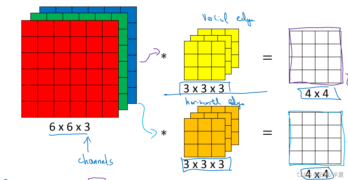
神经网络中的filter （滤波器）与kernel（内核）的概念
kernel: 内核是一个2维矩阵，长 × 宽；
filter：滤波器是一个三维立方体，长× 宽 × 深度，其中深度便是由多少张内核构成；可以说kernel 是filter 的基本元素，多张kernel 组成一个filter。
神经网络中的channels概念
CNN处理过程中，存在输入的channel和输出的channel;其中，输入的channel数=输入数据的深度；输出的channel数=输出数据的深度。

推荐李宏毅的卷积神经网络课：https://www.bilibili.com/video/BV1F4411y7o7?p=7&spm_id_from=pageDriver

tensorflow中的卷积处理函数

tf.nn.conv2d
conv2d(
    input,
    filter,
    strides,
    padding,
    use_cudnn_on_gpu=True,
    data_format='NHWC',
    name=None)
Args:
	• input：输入的tensor，被卷积的图像，conv2d要求input必须是四维的。四个维度分别为[batch, in_height, in_width, in_channels]，
    即batch size，输入图像的高和宽以及单张图像的通道数。
	• filter：卷积核，也要求是四维，[filter_height, filter_width, in_channels, out_channels]四个维度分别表示卷积核的高、宽，输入图像的通道数和卷积输出通道数。
	• strides：步长，即卷积核在与图像做卷积的过程中每次移动的距离，一般定义为[1，stride_h,stride_w,1]，stride_h与stride_w分别表示在高的方向和宽的方向的移动的步长，第一个1表示在batch上移动的步长，最后一个1表示在通道维度移动的步长，而目前tensorflow规定：strides[0] = strides[3] = 1，即不允许跳过bacth和通道，前面的动态图中的stride_h与stride_w均为1
	• padding：边缘处理方式，值为“SAME” 和 “VALID”.
    由于卷积核是有尺寸的，当卷积核移动到边缘时，卷积核中的部分元素没有对应的像素值与之匹配。
    此时选择“SAME”模式，则在对应的位置补零，继续完成卷积运算，在strides为[1,1,1,1]的情况下，卷积操作前后图像尺寸不变即为“SAME”。
    若选择 “VALID”模式，则在边缘处不进行卷积运算，若运算后图像的尺寸会变小。 
Returns:
A Tensor. 4维张量

        self.inputs = tf.p0laceholder(
            shape=[None, 84, 84, 4], dtype=tf.uint8, name="inputs")
        scaled_image = tf.to_float(self.inputs) / 255.0

create_state_network

def state_model(self, input, kernel_shapes, weight_shapes):
        # kernel_shapes=[[8, 8, 4, 32], [4, 4, 32, 64], [3, 3, 64, 64]]
        # [filter_height, filter_width, in_channels, out_channels]
        #  weight_shapes=[[3136, 512]]
        
        weights1 = tf.get_variable(
            "weights1", kernel_shapes[0],
            initializer=tf.contrib.layers.xavier_initializer())
        weights2 = tf.get_variable(
            "weights2", kernel_shapes[1],
            initializer=tf.contrib.layers.xavier_initializer())
        weights3 = tf.get_variable(
            "weights3", kernel_shapes[2],
            initializer=tf.contrib.layers.xavier_initializer())
        weights4 = tf.get_variable(
            "weights5", weight_shapes[0],
            initializer=tf.contrib.layers.xavier_initializer())
        bias1 = tf.get_variable(
            "q_bias1", weight_shapes[0][1],
            initializer=tf.constant_initializer())
        # Convolve
        conv1 = tf.nn.relu(tf.nn.conv2d(
            input, weights1, strides=[1, 4, 4, 1], padding='VALID'))
        conv2 = tf.nn.relu(tf.nn.conv2d(
            conv1, weights2, strides=[1, 2, 2, 1], padding='VALID'))
        conv3 = tf.nn.relu(tf.nn.conv2d(
            conv2, weights3, strides=[1, 1, 1, 1], padding='VALID'))
        # Flatten and Feedforward
        flattened = tf.contrib.layers.flatten(conv3)
        net = tf.nn.relu(tf.nn.xw_plus_b(flattened, weights4, bias1))

        return net

q_model

    def q_model(self, input, weight_shape):
        weights1 = tf.get_variable(
            "q_weights1", weight_shape,
            initializer=tf.contrib.layers.xavier_initializer())
        # 这个初始化器是用来使得每一层输出的方差应该尽量相等。

        bias1 = tf.get_variable(
            "q_bias1", weight_shape[1],
            initializer=tf.constant_initializer())
        # 将变量初始化为给定的常量，初始化一切所提供的值。
        return tf.nn.xw_plus_b(input, weights1, bias1)
    # 计算matmul(input, q_weights1) + q_bias。

b. Prime Network

• Prime Network就是需要被时刻更新的主网络，的主要由create_state_network和target_q_model组成。
• create_state_network和上面的state_network的处理相似，也是将图像经过三层卷积处理然后通过一层全连接层得到观测的状态值。其中，filtersinput的shape两个网络都是一样的。也就是说，两个网络的参数是数量相同且对应的。换言之，create_state_network复制了state_network。
• target_q_model实现了target_Q_out = input * weights1 + bias1，得到了动作价值函数$Q_{\pi }(s,a)$。
• target_network_params 包括了create_state_network里面的参数。target_Q_params包括了weights1 、bias1。
• 用当前网络（State_Network）更新目标网络（Prime_Network）中的参数。tau=0.001。

        self.update_target_network_params = \
            [self.target_network_params[i].assign(
                tf.multiply(self.network_params[i], self.tau) +
                tf.multiply(self.target_network_params[i], 1. - self.tau))
             for i in range(len(self.target_network_params))]

create_state_network

    def create_state_network(self, scaledImage):
        # Convolve
        # kernel_size指的是卷积核的size;stride步长； padding边缘处理方式：'VALID'在边缘处不进行卷积计算
        # out_height = round((in_height - floor(filter_height / 2) * 2) / strides_height) floor表示下取整 round表示四舍五入
        # num_outputs是输出的通道数,等于filters的数量
        # filters:Integer, the dimensionality of the output space (i.e. the number of filters in the convolution).
        conv1 = slim.conv2d(
            inputs=scaledImage, num_outputs=32, kernel_size=[8, 8], stride=[4, 4],
            padding='VALID', biases_initializer=None)
        conv2 = slim.conv2d(
            inputs=conv1, num_outputs=64, kernel_size=[4, 4], stride=[2, 2],
            padding='VALID', biases_initializer=None)
        conv3 = slim.conv2d(
            inputs=conv2, num_outputs=64, kernel_size=[3, 3], stride=[1, 1],
            padding='VALID', biases_initializer=None)
        # Flatten and Feedforward
        flattened = tf.contrib.layers.flatten(conv3)
        net = tf.contrib.layers.fully_connected(
            inputs=flattened,
            num_outputs=self.h_size,
            activation_fn=tf.nn.relu)

        return net

target_q_model

    def target_q_model(self, input, weight_shape):
        weights1 = tf.get_variable(
            "target_q_weights1", weight_shape,
            initializer=tf.contrib.layers.xavier_initializer())
        bias1 = tf.get_variable(
            "target_q_bias1", weight_shape[1],
            initializer=tf.constant_initializer())
        return tf.nn.xw_plus_b(input, weights1, bias1)

c. Action Network

---

• 得到策略价值函数action_probs：${\pi }_{\omega ,\theta }(a|s)$

• 图像经过state_model三层卷积和一层全连接层数量，输出4x4x64个神经元，用于表示图像可观测的状态量。

• 以一层全连接层来对${\pi }_{\omega ,\theta }(a|s)$进行Function Approximation。action_params包括了该全连接层的参数。

• state_out是state_modle的输出，shape=[4,4,64]；action_dim=6; option_dim=8; h_size=512

张量（tensor）运算

算术操作	描述
tf.add(x,y)	将x和y逐元素相加
tf.subtract(x,y)	将x和y逐元素相减
tf.multiply(x,y)	将x和y逐元素相乘
f.divide(x,y)	将x和y逐元素相除
tf.math.mod(x,y)	将x逐元素求余

        self.action_input = tf.concat(
            [self.state_out, self.state_out, self.state_out, self.state_out,
             self.state_out, self.state_out, self.state_out, self.state_out], 1)
        self.action_input = tf.reshape(
            self.action_input, shape=[-1, self.o_dim, 1, self.h_size])
        oh = tf.reshape(self.options_onehot, shape=[-1, self.o_dim, 1])
        self.action_input = tf.reshape(
            tf.reduce_sum(
                tf.squeeze(
                    self.action_input, [2]) * oh, [1]),#行求和
            shape=[-1, 1, self.h_size])
        # tf.reduce_sum 此函数计算一个张量的各个维度上元素的总和.

        self.action_probs = tf.contrib.layers.fully_connected(
            inputs=self.action_input,
            num_outputs=self.a_dim,
            activation_fn=tf.nn.softmax)
        self.action_probs = tf.squeeze(self.action_probs, [1])
        self.action_params = tf.trainable_variables()[
            len(self.network_params) + len(self.target_network_params) +
            len(self.Q_params) + len(self.target_Q_params):]

---

d. Termination Network

• termination_model通过全连接层tf.nn.sigmoid(tf.nn.xw_plus_b(input, weights1, bias1))来对终止函数option_term_prob${\beta }_{\omega ,\vartheta }(s)$进行Function Approximation。
• 神经网络的参数被包括于termination_params中。注意，termination_params和action_params都属于option策略的参数。
• next_option_term_prob表示${\beta }_{\omega ,\vartheta }(s^{{}^{\prime }})$

        with tf.variable_scope("termination_probs") as term_scope:
            self.termination_probs = self.apply_termination_model(
                tf.stop_gradient(self.state_out))# 截断传递的梯度。
            term_scope.reuse_variables()
            self.next_termination_probs = self.apply_termination_model(
                tf.stop_gradient(self.next_state_out))

        self.termination_params = tf.trainable_variables()[-2:]

        self.option_term_prob = tf.reduce_sum(
            self.termination_probs * self.options_onehot, [1])
        self.next_option_term_prob = tf.reduce_sum(
            self.next_termination_probs * self.options_onehot, [1])

        self.reward = tf.placeholder(tf.float32, [None, 1], name="reward")
        self.done = tf.placeholder(tf.float32, [None, 1], name="done")
        # self.disc_option_term_prob = tf.placeholder(tf.float32, [None, 1])

        disc_option_term_prob = tf.stop_gradient(self.next_option_term_prob)

termination_model

    def termination_model(self, input, weight_shape):
        weights1 = tf.get_variable(
            "term_weights1", weight_shape,
            initializer=tf.contrib.layers.xavier_initializer())
        bias1 = tf.get_variable(
            "term_bias1", weight_shape[1],
            initializer=tf.constant_initializer())
        return tf.nn.sigmoid(tf.nn.xw_plus_b(input, weights1, bias1))

e. Actor和Critic网络的更新

• Actor网络的更新上分为两部分：term_gradient表示涉及终止函数的优化目标期望，policy_gradient表示option涉及策略函数的优化目标期望，具体参考下图。
  

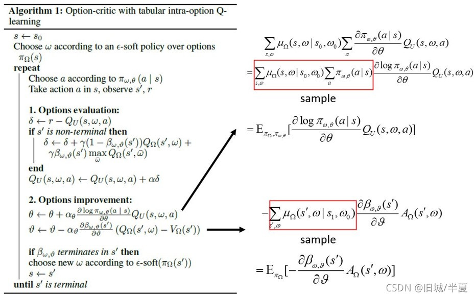
• 但是option策略函数的优化目标函数与算法中的不完全一致，代码中的优化函数加入了action_probs的熵。并将熵的探索率设置为0.01。

 # actor updates
        self.value = tf.stop_gradient(
            tf.reduce_max(self.Q_out, reduction_indices=[1]))

        self.disc_q = tf.stop_gradient(tf.reduce_sum(
            self.Q_out * self.options_onehot, [1]))
        self.picked_action_prob = tf.reduce_sum(
            self.action_probs * self.actions_onehot, [1])
        actor_params = self.termination_params + self.action_params
        # 使用了entropy熵，是否参考了SAC算法？
        entropy = - tf.reduce_sum(self.action_probs *
                                  tf.log(self.action_probs))
        # picked_action_prob为option策略函数
        policy_gradient = - tf.reduce_sum(tf.log(self.picked_action_prob) * y) - \
            entropy_reg * entropy
        # option_term_prob为终止函数
        self.term_gradient = tf.reduce_sum(
            self.option_term_prob * (self.disc_q - self.value))
        self.loss = self.term_gradient + policy_gradient
        grads = tf.gradients(self.loss, actor_params)
        self.actor_updates = tf.train.AdamOptimizer().apply_gradients(zip(grads, actor_params))

• Critic网络更新部分：利用时间差分算法对当前网络的option动作价值 $Q_U(s,\omega )$【在某状态、选择某个option时，采取某行动之后产生的总收益option_Q_out】进行更新。
• 目标网络 option状态价值target_Q_out表示在某状态下选择某个option之后产生的总收益$Q_{\Omega }(s,\omega )$

        '''时间差分算法：
        disc_option_term_prob:终止函数beta
        tf.reduce_sum(self.target_Q_out * self.options_onehot, [1]): option价值函数
        tf.reduce_max(self.target_Q_out, reduction_indices=[1]):计算option最优价值
        self.done:判断s’是否终止，终止为1。
        '''
        y = tf.squeeze(self.reward, [1]) + \
            tf.squeeze((1 - self.done), [1]) * \
            gamma * (
                (1 - disc_option_term_prob) *
                tf.reduce_sum(self.target_Q_out * self.options_onehot, [1]) +
                disc_option_term_prob *
                tf.reduce_max(self.target_Q_out, reduction_indices=[1]))# 计算一个张量的各个维度上元素的最大值.

        y = tf.stop_gradient(y)

        option_Q_out = tf.reduce_sum(self.Q_out * self.options_onehot, [1])# target_Q_out表示的是s'状态的
        td_errors = y - option_Q_out
        # self.td_errors = tf.squared_difference(self.y, self.option_Q_out)
        '''将td_cost分为二次部分和线性部分，但是代码中clip_delta=0，忽略了线性部分'''
        if clip_delta > 0:
            quadratic_part = tf.minimum(abs(td_errors), clip_delta)
            linear_part = abs(td_errors) - quadratic_part
            td_cost = 0.5 * quadratic_part ** 2 + clip_delta * linear_part
        else:
            td_cost = 0.5 * td_errors ** 2

        # critic updates
        '''critic_cost->td_cost-> td_errors->Q_out-> network_params+Q_params
        self.network_params = tf.trainable_variables()[:-2]
        #  三层卷积和全连接层处理，一共有3个卷积核参数+全连接1个权重+全连接1个偏差
        self.Q_params = tf.trainable_variables()[-2:]
        # q_weights1 ,q_bias。'''
        self.critic_cost = tf.reduce_sum(td_cost)
        critic_params = self.network_params + self.Q_params
        grads = tf.gradients(self.critic_cost, critic_params)
        self.critic_updates = tf.train.AdamOptimizer().apply_gradients(zip(grads, critic_params))
        # apply_gradients 使用计算得到的梯度来更新对应的variable.
        # self.critic_updates = tf.train.RMSPropOptimizer(
        #     self.learning_rate, decay=0.95, epsilon=0.01).apply_gradients(zip(grads, critic_params))