深度学习——（8）回归问题

深度学习——（8）回归问题

1.学习目标

掌握搭建pytorch框架的方法，对气温进行预测。

2. 使用数据

百度网盘自取 提取码：hgwt

3.上代码

3.1 相关package

import numpy as np
import pandas as pd 
import matplotlib.pyplot as plt
import torch
import torch.optim as optim
import warnings
warnings.filterwarnings("ignore") # 忽略一些警告
%matplotlib inline # 只在notebook中使用

3.2 数据了解

features = pd.read_csv('temps.csv')
#看看数据长什么样子
features.head()

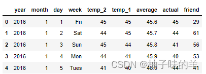
• year,moth,day,week:分别表示的具体的时间
• temp_2：前天的最高温度值
• temp_1：昨天的最高温度值
• average：在历史中，每年这一天的平均最高温度值
• actual：这就是我们的标签值了，当天的真实最高温度
• friend：朋友猜测的可能值，不管就好了

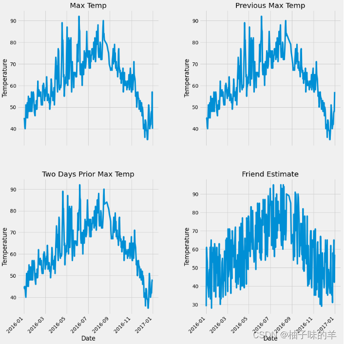
# 画图
# 指定默认风格
plt.style.use('fivethirtyeight')

# 设置布局
fig, ((ax1, ax2), (ax3, ax4)) = plt.subplots(nrows=2, ncols=2, figsize = (15,15)) # 子图布局2*2
fig.autofmt_xdate(rotation = 45) # 横轴倾斜45°

# 标签值
ax1.plot(dates, features['actual'])
ax1.set_xlabel(''); ax1.set_ylabel('Temperature'); ax1.set_title('Max Temp')

# 昨天
ax2.plot(dates, features['temp_1'])
ax2.set_xlabel(''); ax2.set_ylabel('Temperature'); ax2.set_title('Previous Max Temp')

# 前天
ax3.plot(dates, features['temp_2'])
ax3.set_xlabel('Date'); ax3.set_ylabel('Temperature'); ax3.set_title('Two Days Prior Max Temp')

# 我的逗逼朋友
ax4.plot(dates, features['friend'])
ax4.set_xlabel('Date'); ax4.set_ylabel('Temperature'); ax4.set_title('Friend Estimate')

plt.tight_layout(pad=5)# 两图之间的间隔

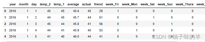
因为week中的是文字，网络不识字，所以换一种编码方式，转换为one-hot形式

# 独热编码 
features = pd.get_dummies(features)
features.head(5)

将数据中的特征和label分开处理

# 标签
labels = np.array(features['actual'])

# 在特征中去掉标签
features= features.drop('actual', axis = 1)

# 名字单独保存一下，以备后患
feature_list = list(features.columns)

# 转换成合适的格式
features = np.array(features)

注！

• 在神经网络中默认值越大参数越重要，所以在训练前要先将数据标准化
• 对所有特征去均值，让数据以原点为中心对称
• 对所有特征除以标准差，将离散范围控制在较小的范围，各个维度上取值范围接近
• 如果某特征全部相等，相当于这一特征对所有结果没有影响

from sklearn import preprocessing
input_features = preprocessing.StandardScaler().fit_transform(features)
input_features[0]

3.3 构建网络模型

后面定义model的时候，不会像下文中那么繁琐，只是为了方便更深刻的理解。

x = torch.tensor(input_features, dtype = float) # 将array中的数据转换为tensor
y = torch.tensor(labels, dtype = float)

# 权重参数初始化，随机初始化
weights = torch.randn((14, 128), dtype = float, requires_grad = True) 
biases = torch.randn(128, dtype = float, requires_grad = True) 
weights2 = torch.randn((128, 1), dtype = float, requires_grad = True) 
biases2 = torch.randn(1, dtype = float, requires_grad = True) 

learning_rate = 0.001 #指定学习率  沿着某个方向到底走多大的步长
losses = [] # 保存损失值

for i in range(1000):  # 迭代1000次
    # 计算隐层
    hidden = x.mm(weights) + biases # 得到中间隐层后要进行一次非线性映射，就是下面的激活函数
    # 加入激活函数
    hidden = torch.relu(hidden)
    # 预测结果
    predictions = hidden.mm(weights2) + biases2 # 得到预测值
    # 通计算损失
    loss = torch.mean((predictions - y) ** 2) #均方误差
    losses.append(loss.data.numpy())# 保存loss用于后期画图，matplot中画图一般是np.array格式
    
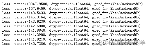
    # 打印损失值
    if i % 100 == 0:
        print('loss:', loss)
    #反向传播计算
    loss.backward()
    
    #更新参数（可以直接调包，为了看到其中真正的原理，下面代码）
    weights.data.add_(- learning_rate * weights.grad.data)  # 沿着权重的反方向去更新，负号的意义
    biases.data.add_(- learning_rate * biases.grad.data)
    weights2.data.add_(- learning_rate * weights2.grad.data)
    biases2.data.add_(- learning_rate * biases2.grad.data)
    
    # 每次迭代都得记得清空  （torch的迭代都是独立的，每一次都要把之前计算出的梯度清零，如果不清零会累加）
    weights.grad.data.zero_()
    biases.grad.data.zero_()
    weights2.grad.data.zero_()
    biases2.grad.data.zero_()

3.4 更简单的构建网络模型

input_size = input_features.shape[1]
hidden_size = 128
output_size = 1
batch_size = 16
my_nn = torch.nn.Sequential( # 序列模块
    torch.nn.Linear(input_size, hidden_size),
    torch.nn.Sigmoid(),# 激活函数
    torch.nn.Linear(hidden_size, output_size),
)
cost = torch.nn.MSELoss(reduction='mean')  # 均值计算损失
optimizer = torch.optim.Adam(my_nn.parameters(), lr = 0.001)
# 训练网络
losses = []
for i in range(1000):
    batch_loss = []
    # MINI-Batch方法来进行训练
    for start in range(0, len(input_features), batch_size):
        end = start + batch_size if start + batch_size < len(input_features) else len(input_features) # 防止越界
        xx = torch.tensor(input_features[start:end], dtype = torch.float, requires_grad = True)
        yy = torch.tensor(labels[start:end], dtype = torch.float, requires_grad = True)
        prediction = my_nn(xx)
        loss = cost(prediction, yy)
        optimizer.zero_grad() # 梯度清零
        loss.backward(retain_graph=True) # 反向传播
        optimizer.step()# 参数更新
        batch_loss.append(loss.data.numpy())
    
    # 打印损失
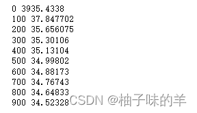
    if i % 100==0:
        losses.append(np.mean(batch_loss))
        print(i, np.mean(batch_loss))

3.5 预测训练结果

x = torch.tensor(input_features, dtype = torch.float)
predict = my_nn(x).data.numpy()

# 转换日期格式
dates = [str(int(year)) + '-' + str(int(month)) + '-' + str(int(day)) for year, month, day in zip(years, months, days)]
dates = [datetime.datetime.strptime(date, '%Y-%m-%d') for date in dates]

# 创建一个表格来存日期和其对应的标签数值
true_data = pd.DataFrame(data = {'date': dates, 'actual': labels})

# 同理，再创建一个来存日期和其对应的模型预测值
months = features[:, feature_list.index('month')]
days = features[:, feature_list.index('day')]
years = features[:, feature_list.index('year')]

test_dates = [str(int(year)) + '-' + str(int(month)) + '-' + str(int(day)) for year, month, day in zip(years, months, days)]

test_dates = [datetime.datetime.strptime(date, '%Y-%m-%d') for date in test_dates]

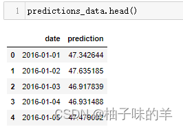
predictions_data = pd.DataFrame(data = {'date': test_dates, 'prediction': predict.reshape(-1)}) 

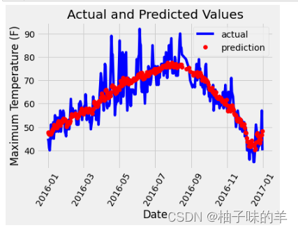
# 真实值
plt.plot(true_data['date'], true_data['actual'], 'b-', label = 'actual')

# 预测值
plt.plot(predictions_data['date'], predictions_data['prediction'], 'ro', label = 'prediction')
plt.xticks(rotation = '60'); 
plt.legend()

# 图名
plt.xlabel('Date'); plt.ylabel('Maximum Temperature (F)'); plt.title('Actual and Predicted Values');