


先看文字版解释相对位置编码解释
visiontransformer中使用到了可学习的绝对位置编码。
swintransformer中将相对值位置编码应用到了图像之中,其中的相对位置代码是通用的,在别的网络中也是这样用的。
1:位置编码应该加在那些地方?
2:位置编码前后的数据流是什么样的?
3:位置编码的代码是如何编写的?
答:
可学习的绝对位置编码在输入图片经过分块后,图片由(B,C,H,W)变成(B,num_patch,emb_dim)后,加上class_token后,加上位置编码。而可学习的编码则是直接初始化为(B,num_patch,emb_dim)大小的0,然后在学习中不断更新。
self.pos_embed = nn.Parameter(torch.zeros(1, num_patches + self.num_tokens, embed_dim))
def forward_features(self, x):
# [B, C, H, W] -> [B, num_patches, embed_dim]
x = self.patch_embed(x) # [B, 196, 768]
# [1, 1, 768] -> [B, 1, 768]
cls_token = self.cls_token.expand(x.shape[0], -1, -1)
if self.dist_token is None:
x = torch.cat((cls_token, x), dim=1) # [B, 197, 768]
else:
x = torch.cat((cls_token, self.dist_token.expand(x.shape[0], -1, -1), x), dim=1)
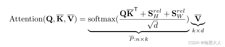
x = self.pos_drop(x + self.pos_embed)而对于相对位置编码:根据公式我们可以看到在Q与K转置相乘后与相对位置编码相加。这里使用Utnet的代码:
import torch
import torch.nn as nn
import torch.nn.functional as F
from einops import rearrange
class depthwise_separable_conv(nn.Module):
    def __init__(self, in_ch, out_ch, stride=1, kernel_size=3, padding=1, bias=False):
        super().__init__()
        self.depthwise = nn.Conv2d(in_ch, in_ch, kernel_size=kernel_size, padding=padding, groups=in_ch, bias=bias, stride=stride)
        self.pointwise = nn.Conv2d(in_ch, out_ch, kernel_size=1, bias=bias)

    def forward(self, x):
        out = self.depthwise(x)
        out = self.pointwise(out)

        return out


class RelativePositionBias(nn.Module):
    # input-independent relative position attention
    # As the number of parameters is smaller, so use 2D here
    # Borrowed some code from SwinTransformer: https://github.com/microsoft/Swin-Transformer/blob/main/models/swin_transformer.py
    def __init__(self, num_heads, h, w):  # (4,16,16)
        super().__init__()
        self.num_heads = num_heads #4
        self.h = h #16
        self.w = w #16

        self.relative_position_bias_table = nn.Parameter(
            torch.randn((2 * h - 1) * (2 * w - 1), num_heads) * 0.02)  # (961,4)

        coords_h = torch.arange(self.h)  # [0,16]
        coords_w = torch.arange(self.w)  # [0,16]
        coords = torch.stack(torch.meshgrid([coords_h, coords_w]))  # (2, 16, 16)
        coords_flatten = torch.flatten(coords, 1)  # (2, 256)

        relative_coords = coords_flatten[:, :, None] - coords_flatten[:, None, :] #(2,256,256)
        relative_coords = relative_coords.permute(1, 2, 0).contiguous() #(256,256,2)
        #转换到大于0
        relative_coords[:, :, 0] += self.h - 1 #(256,256,2)
        relative_coords[:, :, 1] += self.w - 1
        relative_coords[:, :, 0] *= 2 * self.h - 1
        #二维转换到一维
        relative_position_index = relative_coords.sum(-1)  # (256, 256)

        self.register_buffer("relative_position_index", relative_position_index)

    def forward(self, H, W):
        #relative_position_index->(256,256)
        #relative_position_bias_table->(961,4)
        relative_position_bias = self.relative_position_bias_table[self.relative_position_index.view(-1)].view(self.h,self.w,self.h * self.w,-1)  # h, w, hw, nH (16,16,256,4)
        relative_position_bias_expand_h = torch.repeat_interleave(relative_position_bias, H // self.h,dim=0)  # (在dim=0维度重复7次)->(112,16,256,4)
        relative_position_bias_expanded = torch.repeat_interleave(relative_position_bias_expand_h, W // self.w,dim=1)  # HW, hw, nH #(在dim=1维度重复7次)

        relative_position_bias_expanded = relative_position_bias_expanded.view(H * W, self.h * self.w,
                                                                               self.num_heads).permute(2, 0,1).contiguous().unsqueeze(0)

        return relative_position_bias_expanded
class LinearAttention(nn.Module):

    def __init__(self, dim, heads=4, dim_head=64, attn_drop=0., proj_drop=0., reduce_size=16, projection='maxpool',
                 rel_pos=True):
        super().__init__()

        self.inner_dim = dim_head * heads
        self.heads = heads
        self.scale = dim_head ** (-0.5)
        self.dim_head = dim_head
        self.reduce_size = reduce_size
        self.projection = projection
        self.rel_pos = rel_pos

        # depthwise conv is slightly better than conv1x1
        # self.to_qkv = nn.Conv2d(dim, self.inner_dim*3, kernel_size=1, stride=1, padding=0, bias=True)
        # self.to_out = nn.Conv2d(self.inner_dim, dim, kernel_size=1, stride=1, padding=0, bias=True)

        self.to_qkv = depthwise_separable_conv(dim, self.inner_dim * 3)
        self.to_out = depthwise_separable_conv(self.inner_dim, dim)

        self.attn_drop = nn.Dropout(attn_drop)
        self.proj_drop = nn.Dropout(proj_drop)

        if self.rel_pos:
            # 2D input-independent relative position encoding is a little bit better than
            # 1D input-denpendent counterpart
            self.relative_position_encoding = RelativePositionBias(heads, reduce_size, reduce_size)
            # self.relative_position_encoding = RelativePositionEmbedding(dim_head, reduce_size)

    def forward(self, x):
        # x = torch.rand(1,64,112,112)
        B, C, H, W = x.shape

        # B, inner_dim, H, W
        qkv = self.to_qkv(x)  # (1,768,112,112)
        q, k, v = qkv.chunk(3, dim=1)  # (1,256,112,112)

        if self.projection == 'interp' and H != self.reduce_size:
            # 将(k,v)插值到reduce_size大小,(1,256,16,16)
            k, v = map(lambda t: F.interpolate(t, size=self.reduce_size, mode='bilinear', align_corners=True), (k, v))

        elif self.projection == 'maxpool' and H != self.reduce_size:
            k, v = map(lambda t: F.adaptive_max_pool2d(t, output_size=self.reduce_size), (k, v))
        # q--->rearrange--->(1,256(64*4),112,112)->(1,4,12544(112,112),64)
        q = rearrange(q, 'b (dim_head heads) h w -> b heads (h w) dim_head', dim_head=self.dim_head, heads=self.heads,h=H, w=W)
        # k,v--->map--->(1,256(64*4),16,16)->(1,4,256(16,16),64)
        k, v = map(lambda t: rearrange(t, 'b (dim_head heads) h w -> b heads (h w) dim_head', dim_head=self.dim_head,heads=self.heads, h=self.reduce_size, w=self.reduce_size), (k, v))
        # q@k--->(1,4,12544,64)@(1,4,64,256)=(1,4,12544,256)
        q_k_attn = torch.einsum('bhid,bhjd->bhij', q, k)

        if self.rel_pos:
            relative_position_bias = self.relative_position_encoding(H, W)  # (1,4,12544,256)
            q_k_attn += relative_position_bias
            # rel_attn_h, rel_attn_w = self.relative_position_encoding(q, self.heads, H, W, self.dim_head)
            # q_k_attn = q_k_attn + rel_attn_h + rel_attn_w

        q_k_attn *= self.scale
        q_k_attn = F.softmax(q_k_attn, dim=-1)
        q_k_attn = self.attn_drop(q_k_attn)
        #(1,4,12544,256)@(1,4,256,64)=(1,4,12544,64)
        out = torch.einsum('bhij,bhjd->bhid', q_k_attn, v)
        #(1,4,12544,64)--->(1,256(64*4),112,112)
        out = rearrange(out, 'b heads (h w) dim_head -> b (dim_head heads) h w', h=H, w=W, dim_head=self.dim_head,
                        heads=self.heads)
        #(1,256(64*4),112,112)--->(1,64,112,112)
        out = self.to_out(out)
        out = self.proj_drop(out)

        return out, q_k_attn
def main():

#--------------------------------实例化-------------------------
    model = LinearAttention(64) #(传入参数)

    print(model)
    # m = model.state_dict()
    # print(type(m))
    # for key,value in m.items():
    #     print(key)

    model.eval()

    x = torch.rand(1,64,112,112)
    with torch.no_grad():
        output,q_k_attn= model(x)
    print(output.shape) #(1,64,112,112)


if __name__ == '__main__':
    main()
首先我们实例化LinearAttention类,我们输入x,首先获得x的形状,与VisionTransformer不同的是,(VIT首先会进行patchembedding,然后展平,交换维度,然后加入class_token,再加入可学习的位置编码,再经过线性层,最后生成q,k,v),而这里直接经过self.to_qkv函数,即深度可分离函数,升高维度,加入我们x大小为(1,64,112,112),维度变为(1,768,112,112)。
class depthwise_separable_conv(nn.Module):
    def __init__(self, in_ch, out_ch, stride=1, kernel_size=3, padding=1, bias=False):
        super().__init__()
        self.depthwise = nn.Conv2d(in_ch, in_ch, kernel_size=kernel_size, padding=padding, groups=in_ch, bias=bias, stride=stride)
        self.pointwise = nn.Conv2d(in_ch, out_ch, kernel_size=1, bias=bias)

    def forward(self, x):
        out = self.depthwise(x)
        out = self.pointwise(out)

        return out


self.to_qkv = depthwise_separable_conv(dim, self.inner_dim * 3)
然后我们经过chunk函数进行划分,沿着通道维度划分三份,分别为q,k,v的维度,分别为(1,256,112,112)。接着将q,k,v投射或者缩减到我们想要的维度,即(1,256,16,16),然后q经过rearrange函数,由(1256,112,112)转换到(1,4,12544,64)这里和·VIT的类似,都转换到了(B,num_head,HxW,dim_head),k和v转换到由(1,256,16,16)到(1,4,256,16),然后Q乘以K转置,维度变换为q@k--->(1,4,12544,64)@(1,4,64,256)=(1,4,12544,256)。
接着就到了我们的相对位置编码:
这里我们一步一步debug单步调试,看结果的显示
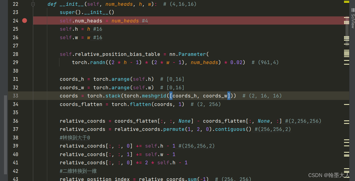
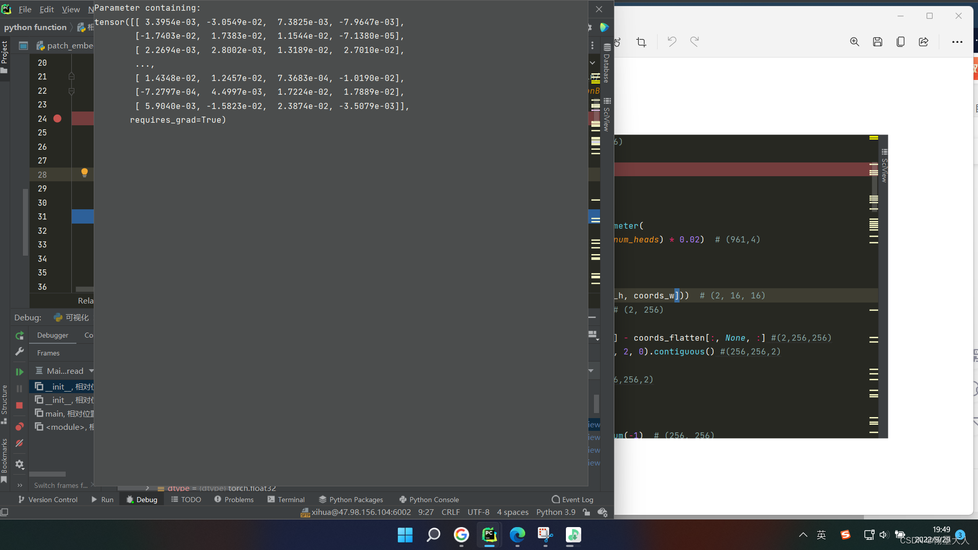
首先h和w都是16,接着我们生成要训练的relative_position_bias_table,这也是我们要用生成的索引去table查找值,具体看文章开头文字版的解释。
我们生成(2M-1)x(2M-1)个值,分别代表行和列,自己的左边和右边共有31个位置一共961个,共有4个头,所以维度为(961,4)。
然以我们生成长和宽的网格用于生成相对位置索引。长和宽都为16

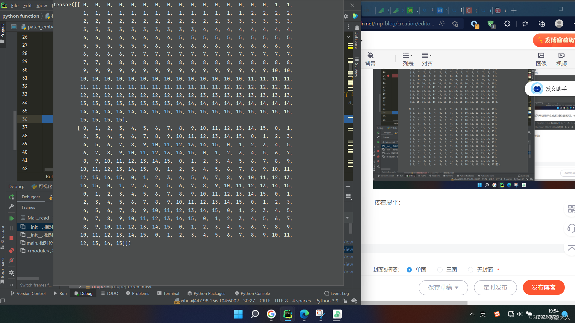
然后meshgrid生成网格:
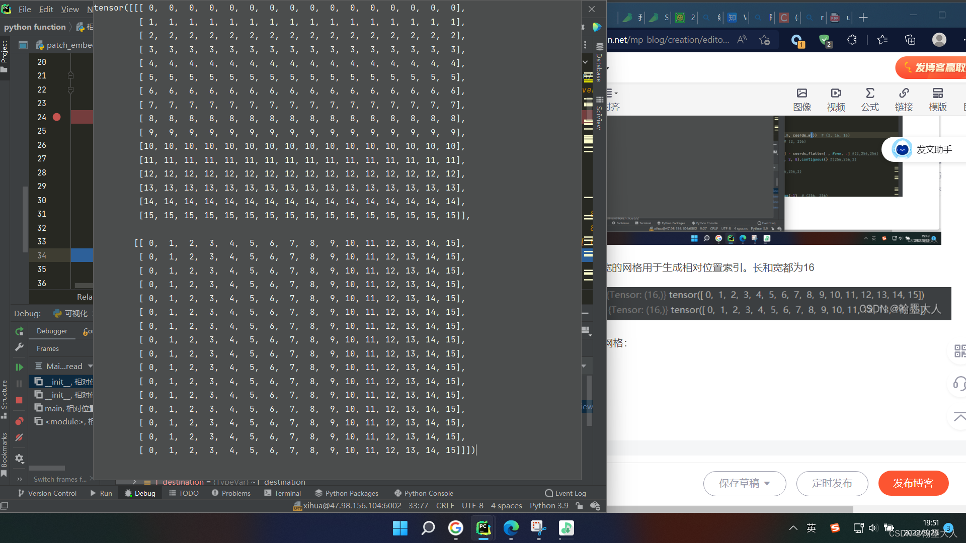
接着展平:
然后获得每个位置的索引:
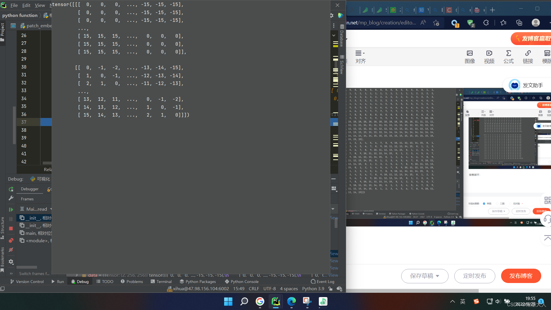
交换维度:
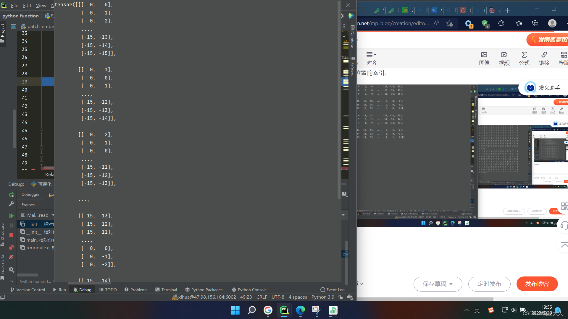
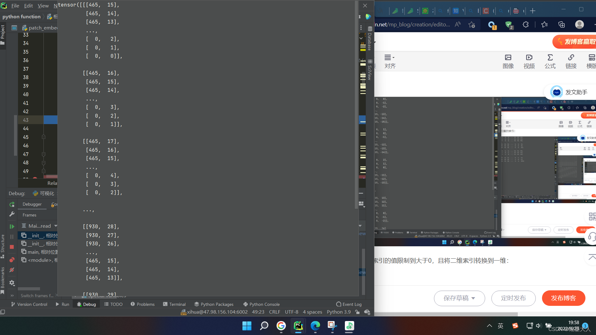
下面的三部将索引的值限制到大于0,且将二维索引转换到一维:
下一步将相对位置索引注册到缓冲区。
在forward函数中,我们将相对位置索引展平,由长和宽拉长为序列,变为
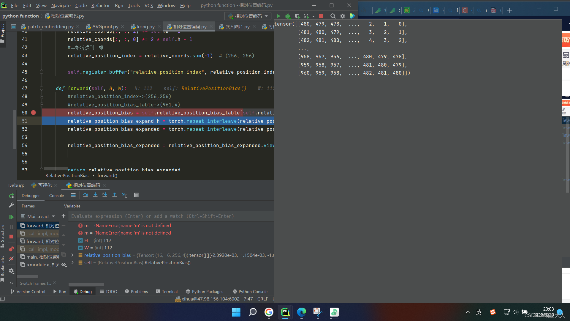
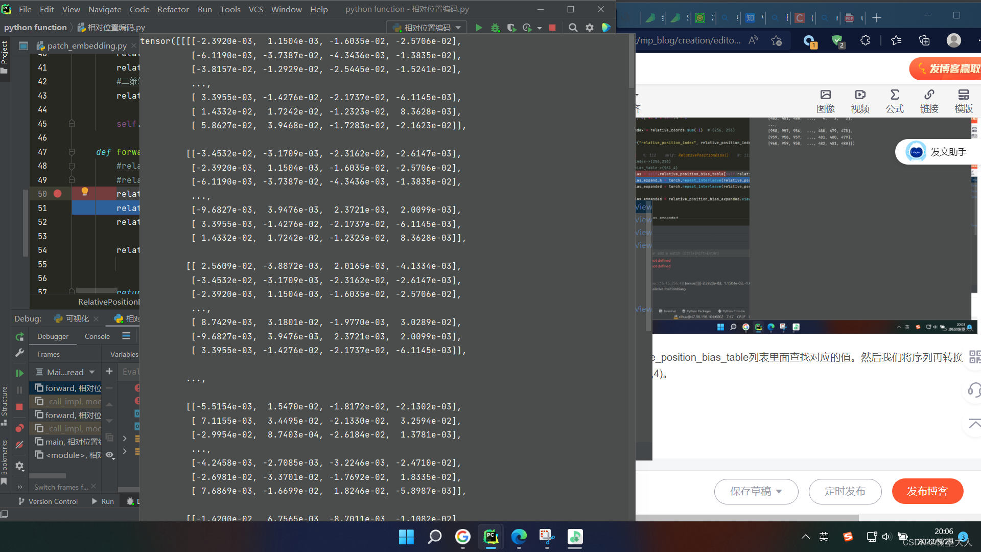
根据生成的索引去relative_position_bias_table列表里面查找对应的值。然后我们将序列再转换到矩阵,大小为 (16,16,256,4)。
由于我们的Q@K大小为(1,4,12544,256),所以我们要将数据进行扩充,长和宽分别扩充七倍。
expand_h为:(112,16,256,4)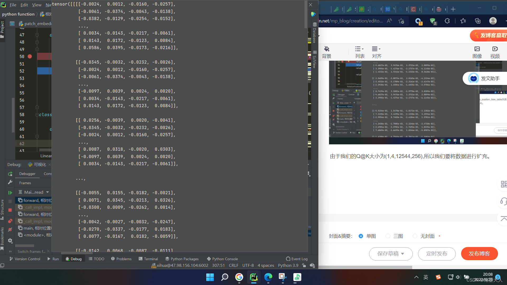
expanded为:(112,112,256,4)
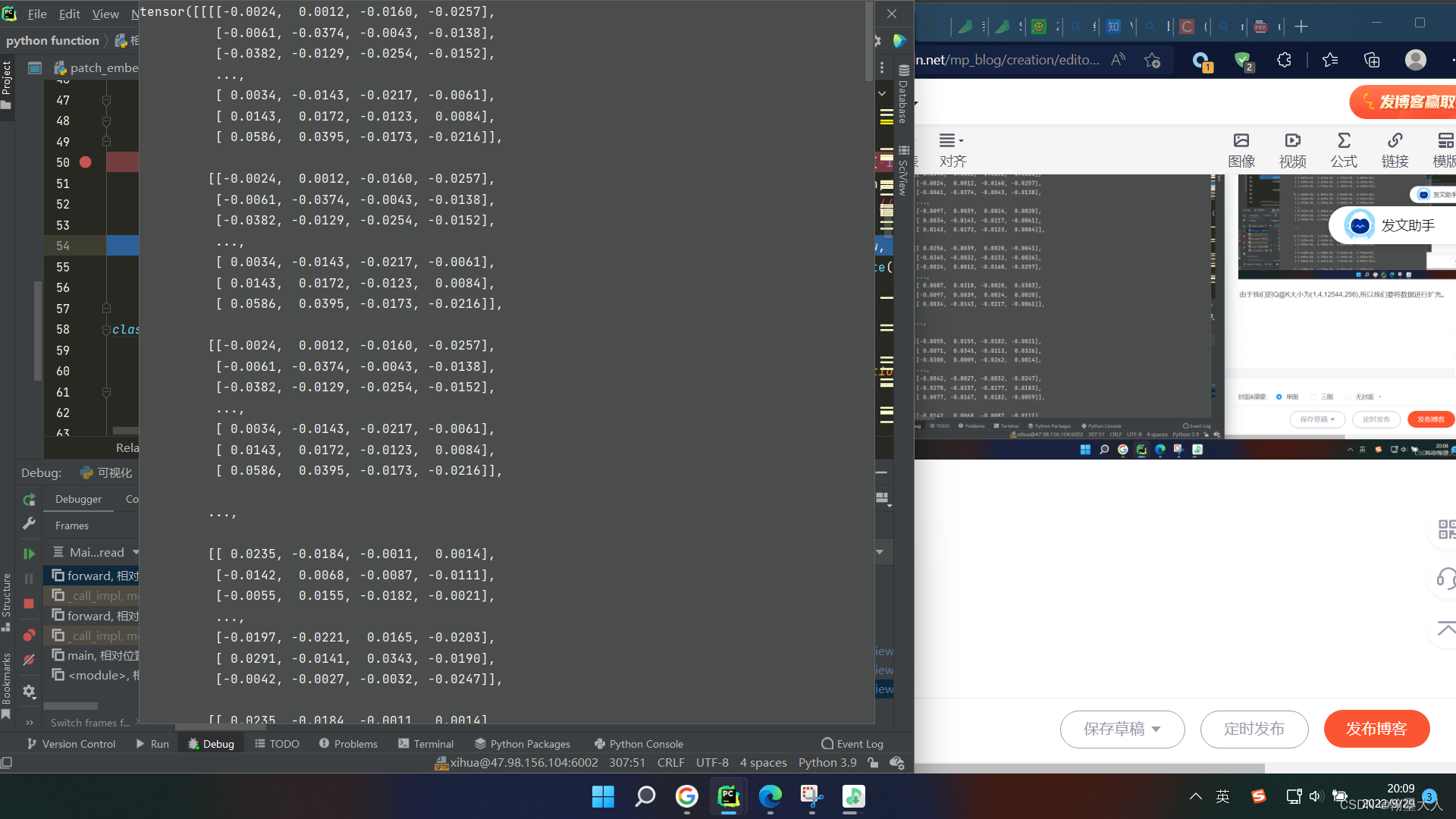
生成的结果进行view,将(112,112,256,4)转换为(1,4,12544,256)。
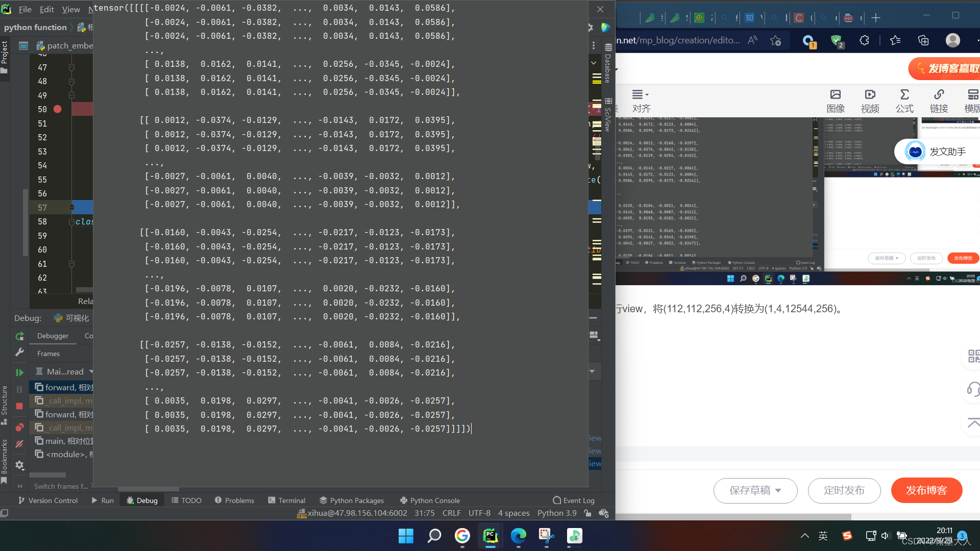
这样我们的bias就与Q@k大小一致了,然后我们相加。接着乘以根号d,在与V相乘。最后reshape为原始大小即可。
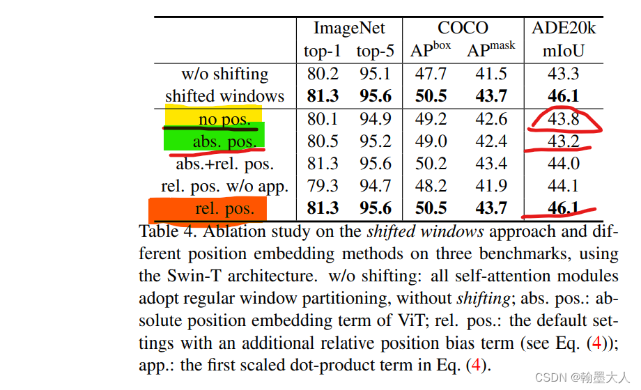
最后我们看一下相对位置编码带来的效果提升:以swintransformer为例:
以语义分割为例,在ADE20K,相对位置编码为46.1,绝对位置编码为43.2,提升了快三个点。究其原因Transformer学到了归纳偏置。


 752
752

 被折叠的 条评论
为什么被折叠?
被折叠的 条评论
为什么被折叠?
 到【灌水乐园】发言


