Reinforcement Learning with Code 【Chapter 5. Monte Carlo Learning】

Reinforcement Learning with Code

This note records how the author begin to learn RL. Both theoretical understanding and code practice are presented. Many material are referenced such as ZhaoShiyu’s Mathematical Foundation of Reinforcement Learning, .

Chapter 5. Monte Carlo Learning

​ What is Monte Carlo estimation? Monte Carlo estimation refers to a broad class of techniques that use stochastic samples to solve approximation problems using the Law of Large Numbers.

​ ChatGpt tells us that “Monte Carlo estimation is a statistical method used to estimate unknown quantities or solve problems by generating random samples and using the law of large numbers to approximate the true value.”

5.1 Law of large numbers

​ (Law of Large Numbers) For a random variable $X$. Suppose { x i } i = 1 n \{x_i\}_{i=1}^n {xi​}i=1n​ are some independent and indentically distribution (iid) samples. Let $\bar{x}=\frac{1}{n}{\sum }_{i=1}^n{x}_i$ be the average of the samples. Then,
$$\begin{gathered} \mathbb{E}[\bar{x}]=\mathbb{E}[X] \\ \mathrm{var}[\bar{x}]=\frac{1}{n}\mathrm{var}[X] \end{gathered}$$
The above two equations indicate that $\bar{x}$ is an unbiased estimate of $\mathbb{E}[X]$ and its variance decreases to zero as $n$ increases to infinity.

​ Proof, First, $\mathbb{E}[\bar{x}]=\mathbb{E}[\frac{1}{n}{\sum }_{i=1}^n{x}_i]=\frac{1}{n}{\sum }_{i=1}^n\mathbb{E}[x_i]=\frac{1}{n}n\mathbb{E}[X]=\mathbb{E}[X]$, where the last equability is because the samples are independent and indentically distribution (iid) (that is, $\mathbb{E}[x_i]=\mathbb{E}[X]$).

​ Second, $\mathrm{var}[\bar{x}]=\mathrm{var}[\frac{1}{n}{\sum }_{i=1}^n{x}_i]=\frac{1}{n^2}{\sum }_{i=1}^n\mathrm{var}[x_i]=\frac{1}{n^2}n\ast \mathrm{var}[X]=\frac{1}{n}\mathrm{var}[X]$, where the second equality is because the samples are independent and indentically distribution (iid) (that is, $\mathrm{var}[x_i]=\mathrm{var}[X]$)

5.2 Simple example

​ Consider a problem that we need to calculate the expectation $\mathbb{E}[X]$ of random variable $X$ which takes value in the finite set $\mathcal{X}$. There are two ways.

​ First, model-based approach, we can use the definition of expectation that
$$\mathbb{E}[X]=\sum _{x\in \mathcal{X}}p(x)x$$
​ Second, model-free approach, if the probability of distribution is unknown we can use the Law of Large Numbers to estimate the expectation.
$$\mathbb{E}[X]\approx \bar{x}=\frac{1}{n}\sum _{i=1}^n{x}_i$$
The example gives us an intutition that: When the system model is available, the expectation can be calculated based on the model.

When the model is unavailable, the expectation can be estimated approximately using stochastic samples.

5.3 Monte Carlo Basic

Review policy iteration:

​ The simplest Monte Carlo learning also called Monte Carlo Basic (MC Basic) just replaces the policy iteration model-based part by MC estimation. Recall the matrix-vector form of policy iteration

$$\begin{array}{rl}{v}_{{\pi }_k}^{(j+1)}& =r_{{\pi }_k}+\gamma P_{{\pi }_k}{v}_{{\pi }_k}^{(j)}\text{(policy evaluation)}\\ {\pi }_{k+1}& =\arg \underset{{\pi }_k}{\max }(r_{{\pi }_k}+\gamma P_{{\pi }_k}{v}_{{\pi }_k})\text{(policy improvement)}\end{array}$$

The elementwise form of policy iteration is

$$\begin{array}{rl}{v}_{{\pi }_k}^{(j+1)}(s)& =\sum _a{\pi }_k(a|s)(\sum _{r}p(r|s,a)r+\sum _{s^{\prime }}p(s^{\prime }|s,a)v_{{\pi }_k}^{(j)}(s^{\prime }))\text{(policy evaluation)}\\ {\pi }_{k+1}(s)& =\arg \underset{{\pi }_k}{\max }\sum _a\pi (a|s)\underset{q_{{\pi }_k}(s,a)}{\underbrace{(\sum _{r}p(r|s,a)r+\sum _{s^{\prime }}p(s^{\prime }|s,a)v_{{\pi }_k}(s^{\prime }))}}\text{(policy improvement)}\\ \to {\pi }_{k+1}(s)& =\sum _a\pi (a|s)\arg \underset{a}{\max }{q}_{{\pi }_k}(s,a)\end{array}$$

Its obvious that the core is to calculate the action values by usting
$$q_{{\pi }_k}(s,a)=\sum _{r}p(r|s,a)r+\sum _{s^{\prime }}p(s^{\prime }|s,a)v_{{\pi }_k}(s^{\prime })$$
​ However, the above equation needs the model of the environment (that $p(r|s,a)$ and $p(s^{\prime }|s,a)$ are required). We can replace this part by Monte Carlo estimation. Recall the definition of action value refer to section 2.5.
$$q_{\pi }(s,a)\triangleq \mathbb{E}[G_t|S_t=s,A_t=a]$$
Action value can be interpreted as average return along trajectory generated by policy $\pi$ after taking a specific action $a$.

Convert to model free:

​ Suppose there are $n$ episodes sampling starting at state $s$ and takeing action $a$, and then denote the $i$ th episode return as $g^{(i)}(s,a)$. Then using the idea of Monte Carlo estimation and Law of Large Numbers, the action values can be approxiamte as
$$q_{\pi }(s,a)\triangleq \mathbb{E}[G_t|S_t=s,A_t=a]\approx \frac{1}{n}\sum _{j=1}^n{g}^{(j)}(s,a)$$
Suppose the number of episodes $n$ is sufficiently large. So, the above equation is the unbiased estimation of action value $q_{\pi }(s,a)$.

Pesudocode:

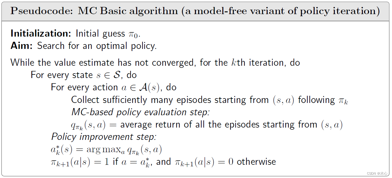
​ Here are some questions. Why does the MC Basic algorithm estimate action values instead of state values? That is because state value cannot be used to improve policies directly. Even if we are given state values, we still need to calculate action values from these state value using $q_{{\pi }_k}(s,a)={\sum }_{r}p(r|s,a)r+{\sum }_{s^{\prime }}p(s^{\prime }|s,a)v_{{\pi }_k}(s^{\prime })$. But this calculation requires the system model. Therefore, when models are not available, we should directly estimate action values.

5.4 Monte Carlo Exploring Starts

Some concepts:

• Vist: a state-action pair appears in the episode, it is called a vist of the state-action pair. Such as
  $$s_1\stackrel{a_2}{\to }{s}_2\stackrel{a_4}{\to }{s}_1\stackrel{a_2}{\to }{s}_2\stackrel{a_3}{\to }{s}_5\stackrel{a_{1}3}{\to }\cdots$$
  $(s_1,a_2)$ is called a visit.

• First visit: In the above trajectory $(s_1,a_2)$ is visited twice. If we only count the first-time visit, such kind of strategy is called first-visit.

• Every visit: If every time state-action pair is visited and the rest of the episode is used to estimate its action value, such a strategy is called every-visit.

​ For example,

$$\begin{array}{rl}{s}_1\stackrel{a_2}{\to }{s}_2\stackrel{a_4}{\to }{s}_1\stackrel{a_2}{\to }{s}_2\stackrel{a_3}{\to }{s}_5\stackrel{a_{1}3}{\to }\cdots & [\text{origianl episode}]\\ s_2\stackrel{a_4}{\to }{s}_1\stackrel{a_2}{\to }{s}_2\stackrel{a_3}{\to }{s}_5\stackrel{a_{1}3}{\to }\cdots & [\text{episode starting from }(s_2,a_4)]\\ s_1\stackrel{a_2}{\to }{s}_2\stackrel{a_3}{\to }{s}_5\stackrel{a_{1}3}{\to }\cdots & [\text{episode starting from }(s_1,a_2)]\\ s_2\stackrel{a_3}{\to }{s}_5\stackrel{a_{1}3}{\to }\cdots & [\text{episode starting from }(s_2,a_3)]\\ s_5\stackrel{a_{1}3}{\to }\cdots & [\text{episode starting from }(s_2,a_4)]\end{array}$$

Suppose we need to estimate the action value $q_{\pi }(s_1,a_2)$. The first-visit only counts the first visit of $(s_1,a_2)$. So we need a huge numbers of episodes starting from $(s_1,a_2)$. As the blue one episode in the above equations. The every-visit counts every time the visit of $(s_1,a_2)$. Hence, we can use the blue one and the red one to estimate the action value $q_{\pi }(s_1,a_2)$. In this way, the samples in the episode are utilized more sufficiently.

Using sample more efficiently:

​ From the example, we are informed that if an episode is sufficiently long so that it can visit all the state-action pairs many times, then this single episode is sufficient to estimate all the action values by using the every-visit strategy. However, one single episode is pretty ideal result. Because the samples obtained by the every-visit is relevant due to the trajectory starting from the second visit is merely a subset of the trajectory starting from the first. Nevertheless, if the two visits are far away from each other, which means there is a siginificant non-overlap portion, the relevance would not be strong. Moreover, the relevance can be further suppressed due to the discount rate. Therefore, when there are few episodes and each episode is very long, the every-visit strategy is a good option.

Using estimation more efficiently:

​ The first startegy in MC Basic, in the policy evaluation step, to collect all the episodes starting from the same state-action pair and then approximate the action value using the average return of these episodes. The drawback of the strategy is that the agent must wait until all episodes have been collected.

​ The second strategy, which can overcome the drawback, is to use the return of a single episode to approximate the corresponding action value (the idea of stochastic estimation). In this way, we can improve the policy in an episode-by-episode fasion.

Pesudocode:

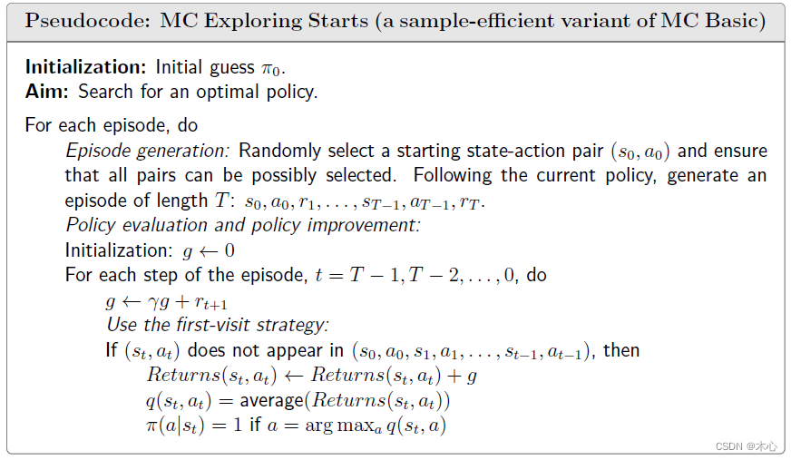
MC Exploring Starts algorithm compared to MC Basic, the sample usage and estimation update are more efficient.

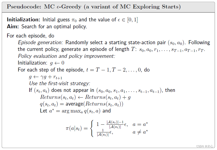
5.5 Monte Carlo $ϵ$-Greedy

​ Why is exploring starts important? In theory, exploring starts is necessary to find optimal policies. Only if every state-action pair is well explored, can we select optimal policies. However, in practice, exploring starts is difficult to achieve. Because its difficult to collect episodes starting from every state-action pair.

​ We can use soft policy to remove the requirement of exploring starts. There are many soft policies. The most common one is $ϵ$-greedy. The $ϵ$-greedy has the form of
$$\pi (a|s)=\{\begin{array}{rl}1-\frac{ϵ}{|\mathcal{A}(s)|}(|\mathcal{A}(s)|-1),& \text{for the geedy action}\\ \frac{ϵ}{|\mathcal{A}(s)|},& \text{for the other }|\mathcal{A}(s)|-1\text{ actions}\end{array}$$
where $|\mathcal{A}(s)|$ denotes the number of actions associated with $s$. It is worth noting taht the probability to take the greedy action is always greater than other action, because
$$1-\frac{ϵ}{|\mathcal{A}(s)|}(|\mathcal{A}(s)|-1)=1-ϵ+\frac{ϵ}{|\mathcal{A}(s)|}\ge \frac{ϵ}{|\mathcal{A}(s)|}$$
for any $ϵ\in [0,1]$, when $ϵ=0$ the $ϵ$-greedy becomes greedy policy.

Pesudocode:

---

Reference

赵世钰老师的课程