Pytorch Tutorial【Chapter 2. Autograd】

Pytorch Tutorial

Chapter 2. Autograd

1. Review Matrix Calculus

1.1 Definition向量对向量求导

​ Define the derivative of a function mapping $f:{\mathbb{R}}^n\to {\mathbb{R}}^m$ as the $n\times m$ matrix of partial derivatives. That is, if $x\in {\mathbb{R}}^n,f(x)\in {\mathbb{R}}^m$, the derivative of $f$ with respect to $x$ is defined as
$${\left[\begin{array}{c}\frac{\partial f}{\partial x}\end{array}\right]}_{ij}=\frac{\partial f_i}{\partial x_i}$$
Let
$$x=\left[\begin{array}{c}{x}_1\\ x_2\\ ⋮\\ x_n\end{array}\right],f(x)=\left[\begin{array}{c}{f}_1(x)\\ f_2(x)\\ ⋮\\ f_m(x)\end{array}\right]$$

then we define the Jacobian Matrix

$$\frac{\partial f}{\partial x}=\left[\begin{array}{cccc}\frac{\partial f_1}{\partial x_1}& \frac{\partial f_2}{\partial x_1}& \cdots & \frac{\partial f_m}{\partial x_1}\\ \frac{\partial f_1}{\partial x_2}& \frac{\partial f_2}{\partial x_2}& \cdots & \frac{\partial f_m}{\partial x_2}\\ ⋮& ⋮& \ddots & ⋮\\ \frac{\partial f_1}{\partial x_n}& \frac{\partial f_2}{\partial x_n}& \cdots & \frac{\partial f_m}{\partial x_n}\end{array}\right]$$

1.2 Definition标量对向量求导

If $f$ is scalar, one has

$$\frac{\partial f}{\partial x}=\left[\begin{array}{c}\frac{\partial f}{\partial x_1}\\ \frac{\partial f}{\partial x_2}\\ ⋮\\ \frac{\partial f}{\partial x_n}\end{array}\right]$$
这其实是一种分母布局

1.3 Definition标量对矩阵求导

​ Now we give some results on the derivative of scalar functions of a matrix. Let $X=[x_{ij}]$ be a matrix of order $m\times n$ and let $y=f(X)$ be a scalar function of $X$. The derivative of $y$ with respect to $X$, denoted by $\frac{\partial y}{\partial X}$, is defined as the following matrix of order $m\times n$,
$$G=\frac{\partial y}{\partial X}=\left[\begin{array}{ccccc}\frac{\partial y}{\partial x_{11}}& \frac{\partial y}{\partial x_{12}}& \cdots & \frac{\partial y}{\partial x_{1n}}& \\ \frac{\partial y}{\partial x_{21}}& \frac{\partial y}{\partial x_{22}}& \cdots & \frac{\partial y}{\partial x_{2n}}& \\ ⋮& ⋮& \ddots & ⋮& \\ \frac{\partial y}{\partial x_{m1}}& \frac{\partial y}{\partial x_{m2}}& \cdots & \frac{\partial y}{\partial x_{mn}}& \end{array}\right]=\left[\frac{\partial y}{\partial x_{ij}}\right]$$

2.关于autograd的说明

torch.Tensor 是包的核心类。如果将其属性 tensor.requires_grad 设置为 True，则会开始跟踪针对 tensor 的所有操作。完成计算后，您可以调用 tensor.backward() 来自动计算所有梯度。该张量的梯度将累积到 tensor.grad 属性中。

要停止 tensor 历史记录的跟踪，您可以调用 tensor.detach()，它将其与计算历史记录分离，并防止将来的计算被跟踪。

要停止跟踪历史记录（和使用内存），您还可以将代码块使用 with torch.no_grad(): 包装起来。在评估模型时，这是特别有用，因为模型在训练阶段具有 requires_grad = True 的可训练参数有利于调参，但在评估阶段我们不需要梯度。

还有一个类对于 autograd 实现非常重要那就是 Function。Tensor 和 Function 互相连接并构建一个非循环图，它保存整个完整的计算过程的历史信息。每个张量都有一个 tensor.grad_fn 属性保存着创建了张量的 Function 的引用，（如果用户自己创建张量，则 grad_fn=None）。

如果你想计算导数，你可以调用 tensor.backward()。如果 Tensor 是标量（即它包含一个元素数据），则不需要指定任何参数backward()，但是如果它有更多元素，则需要指定一个gradient 参数来指定张量的形状。

最后的计算结果保存在tensor.grad属性里

• 使用tensor.requires_grad在初始化时，设置跟踪梯度

import torch
import numpy as np

x = torch.ones(2,2, requires_grad=True)
print(x)

结果如下

tensor([[1., 1.],
        [1., 1.]], requires_grad=True)

• 设置了跟踪梯度的tensor,将会出现tensor.grad_fn的属性，用于记录上次计算的Function

y = torch.add(x, 1)
print(y)
print(y.grad_fn)

结果如下

tensor([[2., 2.],
        [2., 2.]], grad_fn=<AddBackward0>)
<AddBackward0 object at 0x0000020D723EBE80>

• tensor.requires_grad_(True / False) 会改变张量的 requires_grad 标记。 如果没有提供相应的参数输入的标记默认为 False。

a = torch.randn(2,2)
a = (a * 3) / (a-1)
print(a)
a.requires_grad_(True)
print(a)
a = a + 1
print(a)

tensor([[  0.0646, -46.3478],
        [  5.6683,  -0.8896]])
tensor([[  0.0646, -46.3478],
        [  5.6683,  -0.8896]], requires_grad=True)
tensor([[  1.0646, -45.3478],
        [  6.6683,   0.1104]], grad_fn=<AddBackward0>)

3. grad的计算

3.1 Manual手动计算

• 可以使用函数torch.autograd.grad()来手动计算梯度，详细可参考此处

例如计算 $y=x_1^2+x_2^2+x_1{x}_2$的梯度

x1 = torch.tensor(3., requires_grad=True)
x2 = torch.tensor(1., requires_grad=True)
y = x1**2+x2**2+x1*x2

# 求一阶导数
# torch.autograd.grad(y, x1,retain_graph=True, create_graph=True)
x1_1 = torch.autograd.grad(y, x1, retain_graph=True, create_graph=True)[0]
x2_1 = torch.autograd.grad(y, x2, retain_graph=True, create_graph=True)[0]
print(x1_1,x2_1)

# 求二阶混合偏导数
x1_11 = torch.autograd.grad(x1_1, x1)[0]
x1_12 = torch.autograd.grad(x1_1, x2)[0]
x2_21 = torch.autograd.grad(x2_1, x1)[0]
x2_22 = torch.autograd.grad(x2_1, x2)[0]
print(x1_11,x1_12,x2_21,x2_22)

结果如下

tensor(7., grad_fn=<AddBackward0>) tensor(5., grad_fn=<AddBackward0>)
tensor(2.) tensor(1.) tensor(1.) tensor(2.)

3.2 backward()自动计算

当输出是标量scalar函数时
考虑如下的计算问题

x = torch.ones(2,2, requires_grad=True)
y = x + 2
print(y)
z = y * y * 3
out = z.mean()
print(z, out)  #输出out是一个标量
out.backward()
print(x.grad)

输出是

tensor([[3., 3.],
        [3., 3.]], grad_fn=<AddBackward0>)
tensor([[27., 27.],
        [27., 27.]], grad_fn=<MulBackward0>) tensor(27., grad_fn=<MeanBackward0>)
tensor([[4.5000, 4.5000],
        [4.5000, 4.5000]])

$$X=\left[\begin{array}{cc}{x}_1& x_2\\ x_3& x_4\end{array}\right]=\left[\begin{array}{cc}1& 1\\ 1& 1\end{array}\right]$$

中间变量是

$$Z=\left[\begin{array}{cc}{z}_1& z_2\\ z_3& z_4\end{array}\right]=\left[\begin{array}{cc}3(x_1+2{)}^2& 3(x_1+2{)}^2\\ 3(x_1+2{)}^2& 3(x_1+2{)}^2\end{array}\right]$$

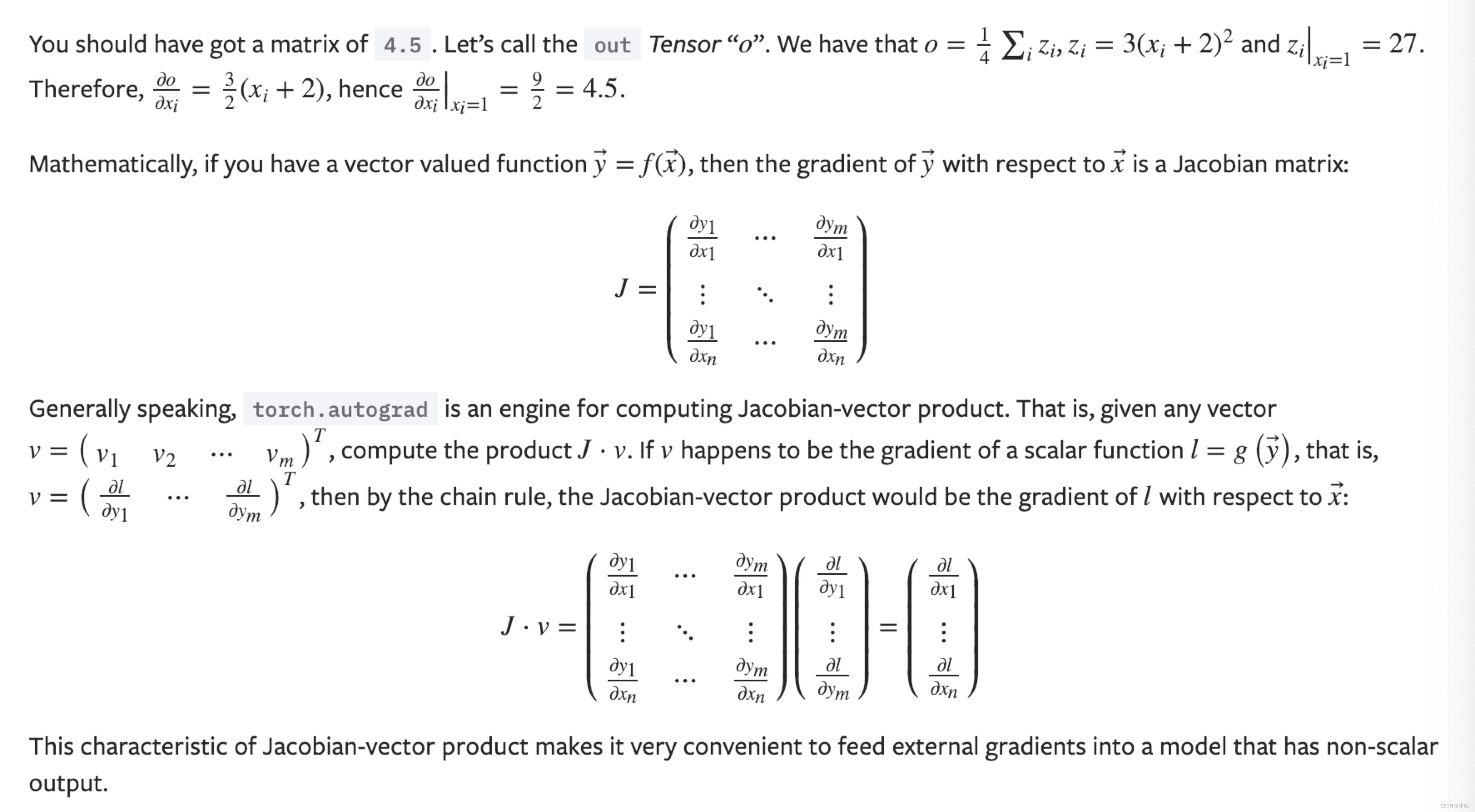
最后获得是输出是

$$\begin{array}{rl}\text{out}& =\frac{1}{4}\sum _{i=1}{z}_i=\frac{1}{4}(z_1+z_2+z_3+z_4)\\ & =\frac{1}{4}(3(x_1+2{)}^2+3(x_2+2{)}^2+3(x_3+2{)}^2+3(x_4+2{)}^2)\\ & =f(\mathrm{x})\end{array}$$

其中将矩阵$X$和矩阵$Z$中的所有元素拼接为向量

$$\begin{gathered} \mathrm{x}=[x_1,x_2,x_3,x_4{]}^T \\ \mathrm{z}=[z_1,z_2,z_3,z_4{]}^T \end{gathered}$$

我们利用矩阵求导的链式法则

$$\frac{\partial f}{\partial \mathrm{x}}=\frac{f(\mathrm{x})}{\partial \mathrm{x}}=\frac{\partial \mathrm{z}}{\partial \mathrm{x}}\frac{\partial f(\mathrm{x})}{\partial \mathrm{z}}$$

再利用标量函数对矩阵导数的定义，则有

$$\frac{\partial f}{\partial \mathrm{x}}=\left[\begin{array}{cccc}\frac{\partial z_1}{\partial x_1}& \frac{\partial z_2}{\partial x_1}& \frac{\partial z_3}{\partial x_1}& \frac{\partial z_4}{\partial x_1}\\ \frac{\partial z_1}{\partial x_2}& \frac{\partial z_2}{\partial x_2}& \frac{\partial z_3}{\partial x_2}& \frac{\partial z_4}{\partial x_2}\\ \frac{\partial z_1}{\partial x_3}& \frac{\partial z_2}{\partial x_3}& \frac{\partial z_3}{\partial x_3}& \frac{\partial z_4}{\partial x_3}\\ \frac{\partial z_1}{\partial x_4}& \frac{\partial z_2}{\partial x_4}& \frac{\partial z_3}{\partial x_4}& \frac{\partial z_4}{\partial x_4}\end{array}\right]\left[\begin{array}{c}\frac{\partial f}{\partial z_1}\\ \frac{\partial f}{\partial z_2}\\ \frac{\partial f}{\partial z_3}\\ \frac{\partial f}{\partial z_4}\end{array}\right]=\left[\begin{array}{cccc}6(x_1+2)& 0& 0& 0\\ 0& 6(x_2+2)& 0& 0\\ 0& 0& 6(x_3+2)& 0\\ 0& 0& 0& 6(x_4+2)\end{array}\right]\left[\begin{array}{c}\frac{1}{4}\\ \frac{1}{4}\\ \frac{1}{4}\\ \frac{1}{4}\end{array}\right]=\left[\begin{array}{c}4.5\\ 4.5\\ 4.5\\ 4.5\end{array}\right]$$

所以最后获得关于的矩阵$X$的导数为

$$\frac{\partial f}{\partial X}=\left[\begin{array}{cc}\frac{\partial f}{\partial x_1}& \frac{\partial f}{\partial x_2}\\ \frac{\partial f}{\partial x_3}& \frac{\partial f}{\partial x_4}\end{array}\right]=\left[\begin{array}{cc}4.5& 4.5\\ 4.5& 4.5\end{array}\right]$$

当输出是张量tensor函数时

x = torch.tensor([[1.0, 2, 3],[4, 5, 6],[7, 8, 9]], requires_grad=True)
w = torch.tensor([[1.0, 2, 3],[4, 5, 6]], requires_grad=True)

y = torch.matmul(x,w.T)
print(y)
print(torch.ones_like(y))
y.backward(gradient = torch.ones_like(y))
print(x.grad)

输出是

tensor([[ 14.,  32.],
        [ 32.,  77.],
        [ 50., 122.]], grad_fn=<MmBackward0>)
tensor([[1., 1.],
        [1., 1.],
        [1., 1.]])
tensor([[5., 7., 9.],
        [5., 7., 9.],
        [5., 7., 9.]])

$$\begin{gathered} Y=X{W}^T \\ \left[\begin{array}{cc}{y}_{11}& y_{21}\\ y_{12}& y_{22}\\ y_{13}& y_{23}\end{array}\right]=\left[\begin{array}{ccc}{x}_{11}& x_{12}& x_{13}\\ x_{21}& x_{22}& x_{23}\\ x_{31}& x_{32}& x_{33}\end{array}\right]\left[\begin{array}{cc}{w}_{11}& w_{21}\\ w_{12}& w_{22}\\ w_{13}& w_{23}\end{array}\right] \\ \left[\begin{array}{cc}{y}_{11}& y_{21}\\ y_{12}& y_{22}\\ y_{13}& y_{23}\end{array}\right]=\left[\begin{array}{cc}(x_{11}{w}_{11}+x_{12}{w}_{12}+x_{13}{w}_{13})& (x_{11}{w}_{21}+x_{12}{w}_{22}+x_{13}{w}_{23})\\ (x_{21}{w}_{11}+x_{22}{w}_{12}+x_{23}{w}_{13})& (x_{21}{w}_{21}+x_{22}{w}_{22}+x_{23}{w}_{23})\\ (x_{31}{w}_{11}+x_{32}{w}_{12}+x_{33}{w}_{13})& (x_{31}{w}_{21}+x_{32}{w}_{22}+x_{33}{w}_{23})\end{array}\right] \end{gathered}$$

gradient=torch.ones_like(y)用于指定矩阵$Y$中每一项的权重都为1，由矩阵$Y$中元素加权得到的scalar函数为

$$\begin{array}{rl}f(\mathrm{x},\mathrm{w})& =1\times y_{11}+1\times y_{12}+1\times y_{13}+1\times y_{21}+1\times y_{22}+1\times y_{23},\\ & \mathrm{x}=[x_{11},x_{12},x_{13},x_{21},x_{22},x_{23},x_{31},x_{32},x_{33}{]}^T\\ & \mathrm{w}=[w_{11},w_{12},w_{13},w_{21},w_{22},w_{23},w_{31},w_{32},w_{33}{]}^T\end{array}$$

这里不包括复合求导，可以直接计算

$$\begin{array}{rl}\frac{\partial f}{\partial \mathrm{x}}& =[\frac{\partial f}{\partial x_{11}},\frac{\partial f}{\partial x_{12}},\frac{\partial f}{\partial x_{13}},\frac{\partial f}{\partial x_{21}},\frac{\partial f}{\partial x_{22}},\frac{\partial f}{\partial x_{23}},\frac{\partial f}{\partial x_{31}},\frac{\partial f}{\partial x_{32}},\frac{\partial f}{\partial x_{33}}{]}^T\\ \frac{\partial f}{\partial \mathrm{x}}& =[w_{11}+w_{21},w_{12}+w_{22},w_{13}+w_{23},w_{11}+w_{21},w_{12}+w_{22},w_{13}+w_{23},w_{11}+w_{21},w_{12}+w_{22},w_{13}+w_{23}{]}^T\\ & =[5,7,9,5,7,9,5,7,9{]}^T\end{array}$$
再写成矩阵的形式则有

$$\frac{\partial f}{\partial X}=\left[\begin{array}{ccc}5& 7& 9\\ 5& 7& 9\\ 5& 7& 9\end{array}\right]$$

再考虑一个更一般求二阶导的情况

x = torch.ones(3, requires_grad=True)
print(x)
y = x * 2
print(y)
z = y * 2
print(z)
v = torch.tensor([0.1, 1.0, 0.0001], dtype=torch.float)
z.backward(gradient=v)
print(x.grad)

结果如下

tensor([1., 1., 1.], requires_grad=True)
tensor([2., 2., 2.], grad_fn=<MulBackward0>)
tensor([4., 4., 4.], grad_fn=<MulBackward0>)
tensor([4.0000e-01, 4.0000e+00, 4.0000e-04])

其中
$$\begin{array}{rl}\mathrm{x}& =[x_1,x_2,x_3{]}^T=[1,1,1{]}^T\\ \mathrm{y}=2\mathrm{x}& =[y_1,y_2,y_3{]}^T=[2,2,2{]}^T\\ \mathrm{z}=2\mathrm{y}& =[z_1,z_2,z_3{]}^T=[4,4,4{]}^T\end{array}$$
若考虑gradient=torch.tensor([a1,a2,a3], dtype=torch.folat)，那么最终加权得到的scalar函数为
$$f=a_1{z}_1+a_2{z}_2+a_3{z}_3$$
那么对$\mathrm{x}$求偏导则有
$$\begin{array}{rl}\frac{\partial f}{\partial \mathrm{x}}& =\frac{\partial \mathrm{y}}{\partial \mathrm{x}}\frac{\partial f}{\partial \mathrm{y}}\\ & =\left[\begin{array}{ccc}\frac{\partial y_1}{\partial x_1}& \frac{\partial y_2}{\partial x_1}& \frac{\partial y_3}{\partial x_1}\\ \frac{\partial y_1}{\partial x_2}& \frac{\partial y_2}{\partial x_2}& \frac{\partial y_3}{\partial x_2}\\ \frac{\partial y_1}{\partial x_3}& \frac{\partial y_2}{\partial x_3}& \frac{\partial y_3}{\partial x_3}\end{array}\right]\left[\begin{array}{c}\frac{\partial f}{\partial y_1}\\ \frac{\partial f}{\partial y_2}\\ \frac{\partial f}{\partial y_3}\end{array}\right]\\ & =\left[\begin{array}{ccc}2& & \\ & 2& \\ & & 2\end{array}\right]\left[\begin{array}{c}2a_1\\ 2a_2\\ 2a_3\end{array}\right]\\ & =[4a_1,4a_2,4a_3{]}^T\end{array}$$

一些启示

---

Reference

参考教程1
参考教程2