项目实战｜手把手教你实现病理切片染色标准化｜项目复现·24-08-30

小罗碎碎念

本期推文主题：手把手教你完成病理切片的染色标准化

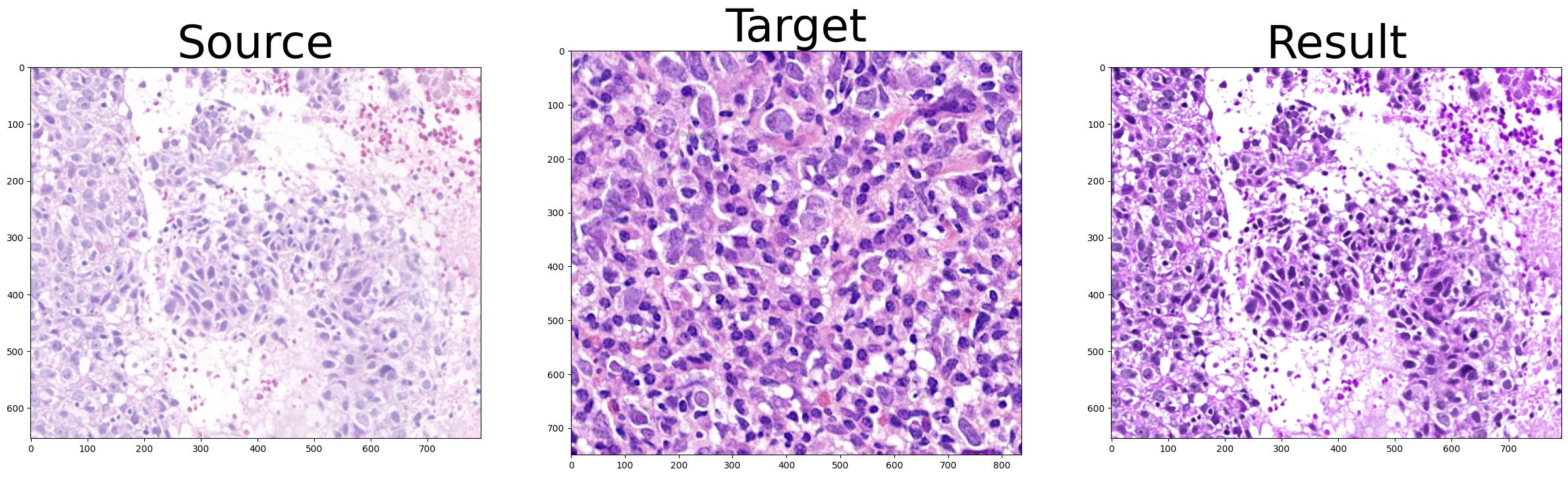
阅读完本期推文以后，你能实现的效果如下。

友情提醒，本教程仅适用于Mac和Linux用户，Windows用户无法下载关键的包spams。

---

参考资料

https://github.com/xindubawukong/Vahadane

https://blog.csdn.net/qq_45654306/article/details/125082904?spm=1001.2014.3001.5506

---

一、导入包&配置路径

import numpy as np
import matplotlib.pyplot as plt
import spams
import cv2
import utils
from vahadane import vahadane
from sklearn.manifold import TSNE

%load_ext autoreload
%autoreload 2
%matplotlib inline

SOURCE_PATH = './data/SMU.jpg'
TARGET_PATH = './data/SYSUCC.jpg'
RESULT_PATH = './output'

---

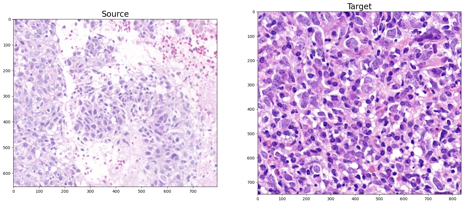
二、加载原图像和目标图像

source_image = utils.read_image(SOURCE_PATH)
target_image = utils.read_image(TARGET_PATH)
print('source image size: ', source_image.shape)
print('target image size: ', target_image.shape)
plt.figure(figsize=(20.0, 20.0))
plt.subplot(1, 2, 1)
plt.title('Source', fontsize=20)
plt.imshow(source_image)
plt.subplot(1, 2, 2)
plt.title('Target', fontsize=20)
plt.imshow(target_image)
plt.show()

# 结果，别复制
source image size:  (654, 794, 3)
target image size:  (750, 836, 3)

---

三、更改配置

vhd = vahadane(LAMBDA1=0.01, LAMBDA2=0.01, fast_mode=1, getH_mode=0, ITER=50)
vhd.show_config()

# 结果，别复制
STAIN_NUM = 2
THRESH = 0.9
LAMBDA1 = 0.01
LAMBDA2 = 0.01
ITER = 50
fast_mode = 1
getH_mode = 0

---

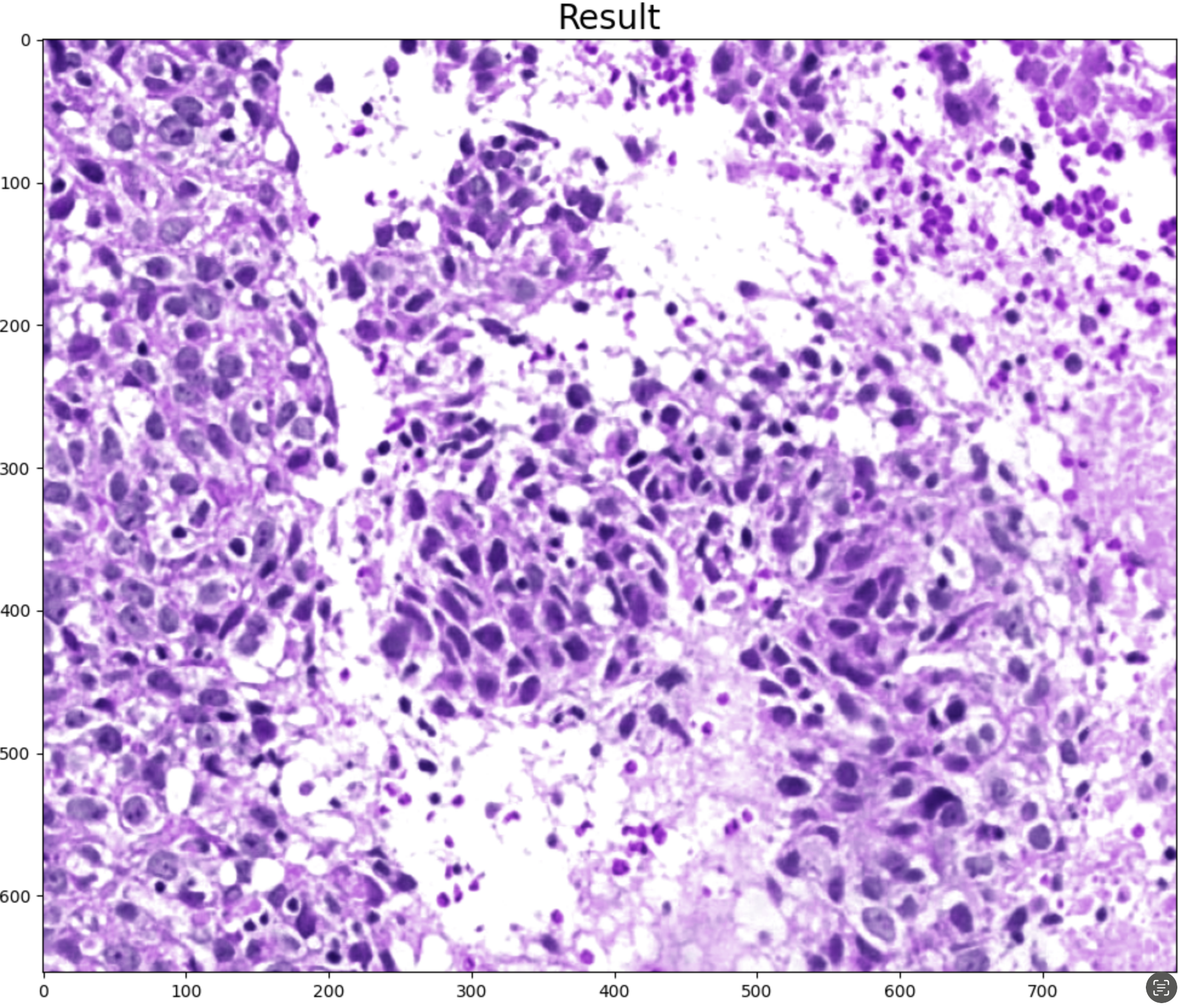
四、染色分离&染色标准化

Ws, Hs = vhd.stain_separate(source_image)
vhd.fast_mode=0;vhd.getH_mode=0;
Wt, Ht = vhd.stain_separate(target_image)

# 结果，别复制
stain separation time: 0.3468461036682129 s
stain separation time: 0.20299434661865234 s

---

img = vhd.SPCN(source_image, Ws, Hs, Wt, Ht)
plt.figure(figsize=(20.0, 10.0))
plt.title('Result', fontsize=20)
plt.imshow(img)
plt.show()
cv2.imwrite(RESULT_PATH, cv2.cvtColor(img, cv2.COLOR_RGB2BGR))

---

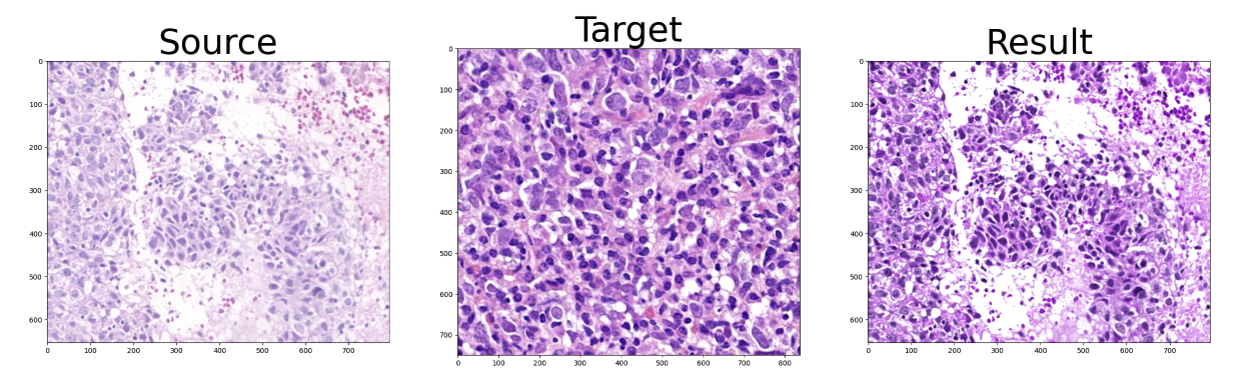
plt.figure(figsize=(30, 10))
plt.subplot(1,3,1)
plt.title('Source', fontsize=50)
plt.imshow(source_image)
plt.subplot(1,3,2)
plt.title('Target', fontsize=50)
plt.imshow(target_image)
plt.subplot(1,3,3)
plt.title('Result', fontsize=50)
plt.imshow(img)
plt.savefig(RESULT_PATH)
plt.show()
  

---

tsne = TSNE(n_components=2, init='pca', random_state=19980723)
data = np.concatenate((img[:, :, 0], img[:, :, 1], img[:, :, 2]), axis=0)
print(data.shape)
result = tsne.fit_transform(data.T)
print(result)

# 结果，别复制
(1962, 794)
[[-35.462708    -9.232457  ]
 [-35.230995    -9.582003  ]
 [-34.833885   -10.199884  ]
 ...
 [ -3.534977     1.4352764 ]
 [ -4.226372     1.2181394 ]
 [ -4.2816014    0.78518176]]

---

data = np.concatenate((source_image[:,:,0],source_image[:,:,1],source_image[:,:,2]), axis=0)
print(data.shape)
result0 = tsne.fit_transform(data.T)
print(result0)

# 结果，别复制
(1962, 794)
[[-32.603973   -2.50919  ]
 [-32.739643   -2.9601758]
 [-32.94034    -3.6632967]
 ...
 [  0.4973097   6.99416  ]
 [  0.4592985   6.269702 ]
 [  0.8823547   6.0223703]]

---

t_min = result.min(axis=0)
t_max = result.max(axis=0)
result = (result - t_min) / (t_max - t_min)
t_min = result0.min(axis=0)
t_max = result0.max(axis=0)
result0 = (result0 - t_min) / (t_max - t_min)
print(result)
print(result0)
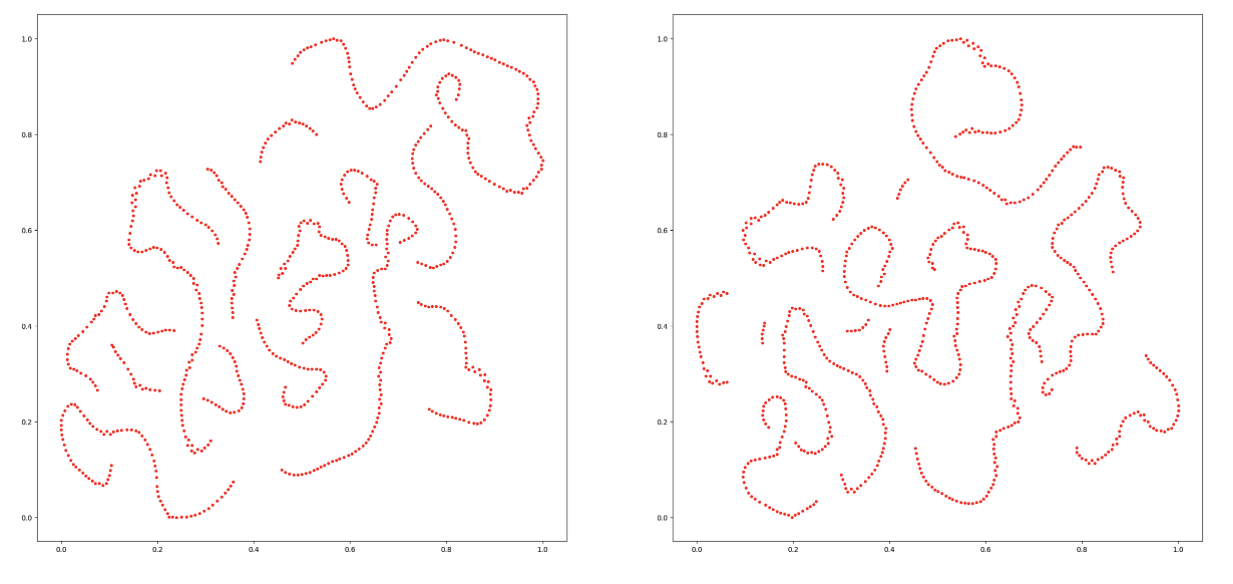
plt.figure(figsize=(30, 30))
plt.subplot(2,2,1)
plt.plot(result[:, 0], result[:, 1], 'r.')
plt.subplot(2,2,2)
plt.plot(result0[:,0], result0[:,1], 'r.')
plt.show()

# 结果，别复制
[[0.1056293  0.36017856]
 [0.10819688 0.35528234]
 [0.11259724 0.34662744]
 ...
 [0.45941886 0.5096052 ]
 [0.45175755 0.5065637 ]
 [0.45114556 0.5004991 ]]
[[0.1406844  0.40613082]
 [0.13925514 0.40020835]
 [0.13714086 0.39097482]
 ...
 [0.48939934 0.53093106]
 [0.4889989  0.5214173 ]
 [0.4934557  0.5181693 ]]