使用mathematica探究立方体与平面求交的性质

最新推荐文章于 2024-05-04 10:17:43 发布

qq_45769623

最新推荐文章于 2024-05-04 10:17:43 发布

阅读量315

点赞数

文章标签： matlab Powered by 金山文档

本文链接：https://blog.csdn.net/qq_45769623/article/details/128697776

版权

问题的起源来源于我要比较 $\text{[math]}$ 和 $\text{[math]}$ 的大小进而得到一些条件，关于函数 $\text{[math]}$ 最后再说。

如图，立方体中心为原点，边长为2，平面过原点，两者交于一个凸多边形。凸多边形一点到原点的距离记为 $\text{[math]}$ ,我要考虑 $\text{[math]}$ 的性质，先根据导数的定义（实际可以直接由上图右得到），得到 $\text{[math]}$ $\text{[math]}$ 。于是探究随着平面法向变化多边形内角的性质。

首先使用Manipulate可视化：

Animate[Graphics3D[Cuboid[{-1, -1, -1}, {1, 1, 1}], Axes -> True, 
  AxesLabel -> {x, y, z}, 
  ClipPlanes -> -{ Sin[theta] Cos[phi], Sin[theta] Sin[phi], 
     Cos[theta], 0}, Boxed -> False, 
  ClipPlanesStyle -> 
   Directive[Yellow, Opacity[0.5], Specularity[White, 30]]], {{theta, 
   Pi/2}, 0, Pi/2, Appearance -> "Labeled"}, {{phi, Pi/4}, 0, Pi, 
  Appearance -> "Labeled"}, AnimationRunning -> False]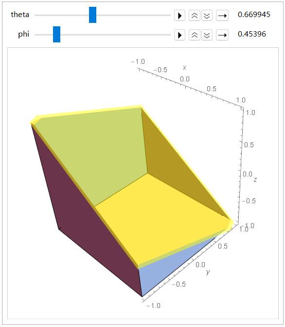

了解性质后，考虑如何求出交得的多边形。

首先，由于立方体表面公式为||x-y|+|x+y|-2z|+||x-y|+|x+y|+2z|=4，直接与平面联立使用Solve求解，求解出结果过于复杂。

采取另一种方法，取出立方体边界线框，使用RegionIntersection求出平面与所有线段的交点（开始时我求平面与所有表面的交集再取交点，存在由于舍入误差而重复的交点），再对交点集去除重复，再进行仿射变换投影回二维平面，再对顶点进行排序，（已知顶点集合时排序时使用Shortestdistance十分好用）排序后顶点组成多边形，计算每个顶点周围两个夹角的 $\text{[math]}$ 值，与 $\text{[math]}$ 的最大值作比较，统计大于该值的顶点个数，作为函数输出。

lines = MeshPrimitives[Cuboid[{-1, -1, -1}, {1, 1, 1}], 1];
poins322[{x_, y_, z_}] := {x, y}
caltan[p1_, p2_, p3_] := 
 Module[{vec1 = -p2, vec2 = p1 - p2, vec3 = p3 - p2}, 
  Max[Abs[Tan[ArcCos[Dot[vec1, vec2]]]], 
   Abs[Tan[ArcCos[Dot[vec1, vec3]]]]]]
number1[list_] := 
 Module[{length = Length[list], ans = 0.}, 
  For[i = 1, i <= length, 
   ans = If[
     caltan[list[[Mod[i - 1, length, 1]]], list[[Mod[i, length, 1]]], 
       list[[Mod[i + 1, length, 1]]]] < 1./0.35355, ans + 1., ans], 
   i++]; ans]
number[theta_, phi_] := 
 Block[{a = Sin[theta] Cos[phi], b = Sin[theta] Sin[phi], 
   c = Cos[theta], plane1, pts, r, pts1, pts2, ordList}, 
  plane1 = Hyperplane[{a, b, c}, {0., 0., 0.}];
  pts = RegionIntersection[#, plane1] & /@ lines; 
  pts = DeleteCases[pts, EmptyRegion[3]];
  pts = First /@ First /@ pts;
  r = RotationTransform[{{a, b, c}, {0, 0, 1}}, {0, 0, 0}];
  pts1 = r[#] & /@ pts ;
  pts2 = poins322[#] & /@ pts1;
  ordList = SortBy[pts2, Apply[N[ArcTan[#1, #2]] &]];
  number1[ordList]]
number[0., 0.] // AbsoluteTiming
(*Plot3D[number[u,v],{u,0,Pi},{v,0,2 \
Pi},PlotPoints\[Rule]10]//AbsoluteTiming*)

ParametricPlot3D[{Sin[\[Theta]] Cos[\[Phi]], 
   Sin[\[Theta]] Sin[\[Phi]], Cos[\[Theta]]}, {\[Theta], 
   0, \[Pi]/2}, {\[Phi], 0, \[Pi]/2}, PlotPoints -> 50, 
  PerformanceGoal -> "Quality", 
  ColorFunction -> 
   Function[{x, y, z, \[Theta], \[Phi]}, 
    Hue[number[\[Theta], \[Phi]]/12]], 
  ColorFunctionScaling -> False] // AbsoluteTiming

由于采用ParametricPlot3D，并在每点的颜色上设定函数，我的求交点个数函数中RegionIntersection函数会花费0.016s时间导致画图效率十分低。尽管我后来加大plotpoints的数值，减小lines里边的个数，只绘制1/16的球面再通过仿射变换绘制整个球面，绘制出来的结果仍然不精美。

当平面法向取遍球面时，画出如下结果：

使用解析方法，我开始求上面球面上的曲线的解析表达式。取定球面在第一象限的一小部分，此时平面与球的交点会在三条已知的线段上，设交点的坐标为变量，对交点的夹角正切值进行绘制：

可以直接判断大小，再逐个判断哪个点的哪个夹角更小。由于交点坐标可以写为平面法向的分量的表达式，带入平面法向，计算得，

$\text{[math]}$ ,其中k为关于函数d的值。

至此，我需要在球面上绘制出上式与

$\text{[math]}$ 所围成的区域。

开始时我想要通过ImplicitRegion画出定义域，确实可以根据几个不等式确定，然而，通过隐式区域画出的图片也不好看，也是由于逐点绘制的原因。

后来我使用球面坐标， $\text{[math]}$ 进而化简为

$\text{[math]}$ 的形式，使用Reduce求出 $\text{[math]}$ 关于 $\text{[math]}$ 的表达式，在球面上paramatricPlot画出曲线。

solve求解出各线的交点，再根据围成的区域绘制各个小区面：（需要注意的是有些曲线在某处无定义，需要在分割曲线）

opsity = 1;
spe = 100;

kb = 1.2;
k = 1/2 (Sqrt[kb] - 1/Sqrt[kb])
npoints = 30;
theta1[phi_] := 
  2 (ArcTan[(-1 - Tan[phi/2]^2 + Sqrt[
      1 - k^2 + 6 Tan[phi/2]^2 + 2 k^2 Tan[phi/2]^2 + Tan[phi/2]^4 - 
       k^2 Tan[phi/2]^4])/(-k + 2 Tan[phi/2] + k Tan[phi/2]^2)]);
theta2[phi_] := 
  2 (ArcTan[(-1 - Tan[phi/2]^2 - Sqrt[
      1 - k^2 + 6 Tan[phi/2]^2 + 2 k^2 Tan[phi/2]^2 + Tan[phi/2]^4 - 
       k^2 Tan[phi/2]^4])/(-k + 2 Tan[phi/2] + k Tan[phi/2]^2)]);
theta3[phi_] := 
  2 (ArcTan[(
     1 + Tan[phi/2]^2 - 
      Sqrt[2] Sqrt[1 - 2 k^2 Tan[phi/2]^2 + Tan[phi/2]^4])/(-1 + 
      2 k Tan[phi/2] + Tan[phi/2]^2)]);
theta4[phi_] := 
  2 (ArcTan[(
     1 + Tan[phi/2]^2 + 
      Sqrt[2] Sqrt[1 - 2 k^2 Tan[phi/2]^2 + Tan[phi/2]^4])/(-1 + 
      2 k Tan[phi/2] + Tan[phi/2]^2)]);
theta5[phi_] := -2 ArcTan[
    Cos[phi] + Sin[phi] + Sqrt[
     1 + Cos[phi]^2 + 2 Cos[phi] Sin[phi] + Sin[phi]^2]];
theta6[phi_] := -2 ArcTan[
    Cos[phi] + Sin[phi] - Sqrt[
     1 + Cos[phi]^2 + 2 Cos[phi] Sin[phi] + Sin[phi]^2]];
theta7[phi_] := -2 ArcTan[Cos[phi] + Sqrt[1 + Cos[phi]^2]];
theta8[phi_] := -2 ArcTan[Cos[phi] - Sqrt[1 + Cos[phi]^2]];
phi38 = x /. 
  FindRoot[(
    1 + Tan[x/2]^2 - 
     Sqrt[2] Sqrt[1 - 2 k^2 Tan[x/2]^2 + Tan[x/2]^4])/(-1 + 
     2 k Tan[x/2] + Tan[x/2]^2) == -Cos[x] + Sqrt[1 + Cos[x]^2], {x, 
    Pi/4}]
phi16 = x /. 
  FindRoot[(-1 - Tan[x/2]^2 + Sqrt[
     1 - k^2 + 6 Tan[x/2]^2 + 2 k^2 Tan[x/2]^2 + Tan[x/2]^4 - 
      k^2 Tan[x/2]^4])/(-k + 2 Tan[x/2] + k Tan[x/2]^2) == -Cos[x] - 
     Sin[x] + Sqrt[1 + Cos[x]^2 + 2 Cos[x] Sin[x] + Sin[x]^2], {x, 
    Pi/4}]
phi16d = x /. FindRoot[-k + 2 Tan[x/2] + k Tan[x/2]^2 == 0, {x, phi16}]
If[phi16 > phi16d, phi16d = phi16 - 0.001];
piece48 = Show[
  (*ParametricPlot3D[{{Sin[theta1[phi]] Cos[phi],Sin[theta1[phi]] Sin[
  phi],Cos[theta1[phi]]},{Sin[theta3[phi]] Cos[phi],Sin[theta3[
  phi]] Sin[phi],Cos[theta3[phi]]},(*{Sin[theta4[phi]] Cos[phi],Sin[
  theta4[phi]] Sin[phi],Cos[theta4[phi]]},{Sin[theta5[phi]] Cos[phi],
  Sin[theta5[phi]] Sin[phi],Cos[theta5[phi]]},*){Sin[theta6[phi]] Cos[
  phi],Sin[theta6[phi]] Sin[phi],Cos[theta6[phi]]},{Sin[theta8[
  phi]] Cos[phi],Sin[theta8[phi]] Sin[phi],Cos[theta8[phi]]}},{phi,
  phi16,Pi/4},PlotLegends\[Rule]{1,3,6,8},PlotRange\[Rule]All],*)
  
  ParametricPlot3D[{ Sin[t theta6[phi] + (1 - t) 0]  Cos[phi], 
    Sin[t theta6[phi] + (1 - t) 0] Sin[phi], 
    Cos[t theta6[phi] + (1 - t) 0] },(*Element[{u,v},
   region1]*){t, 0, 1}, {phi, 0, Pi/4}, 
   PlotPoints -> {npoints, npoints}, Mesh -> None, 
   PlotStyle -> 
    Directive[Opacity[opsity](*, Specularity[White,spe]*)], 
   PlotTheme -> "BoldColor"],
  ParametricPlot3D[{ 
    Sin[t theta6[phi] + (1 - t) theta8[phi]] Cos[phi], 
    Sin[t theta6[phi] + (1 - t) theta8[phi]]  Sin[phi], 
    Cos[t theta6[phi] + (1 - t) theta8[phi]]},(*Element[{u,v},
   region1]*){t, 0, 1}, {phi, 0, phi38}, 
   PlotPoints -> {npoints, npoints}, Mesh -> None, 
   PlotStyle -> 
    Directive[Opacity[opsity](*, Specularity[White,spe]*)], 
   PlotTheme -> "BoldColor"],
  ParametricPlot3D[{ 
    Sin[t theta6[phi] + (1 - t) theta3[phi]] Cos[phi], 
    Sin[t theta6[phi] + (1 - t) theta3[phi]]  Sin[phi], 
    Cos[t theta6[phi] + (1 - t) theta3[phi]]},(*Element[{u,v},
   region1]*){t, 0, 1}, {phi, phi38, phi16}, 
   PlotPoints -> {npoints, npoints}, Mesh -> None, 
   PlotStyle -> 
    Directive[Opacity[opsity](*, Specularity[White,spe]*)], 
   PlotTheme -> "BoldColor"],
  (*ParametricPlot3D[{ Sin[t theta8[phi]+(1-t) theta1[phi]] Cos[phi], 
  Sin[t theta8[phi]+(1-t) theta1[phi]]  Sin[phi],Cos[t theta8[phi]+(1-
  t) theta1[phi]]},(*Element[{u,v},region1]*){t,0,1},{phi,phi16,
  phi16d},PlotPoints\[Rule]{npoints,npoints},Mesh\[Rule]None,
  PlotStyle\[Rule]Directive[Opacity[opsity](*, Specularity[White,
  spe]*)],PlotTheme->"BoldColor"],*)
  (*ParametricPlot3D[{ Sin[t theta8[phi]+(1-t) theta1[phi]] Cos[phi], 
  Sin[t theta8[phi]+(1-t) theta1[phi]]  Sin[phi],Cos[t theta8[phi]+(1-
  t) theta1[phi]]},(*Element[{u,v},region1]*){t,0,1},{phi,phi16d,
  phi38},PlotPoints\[Rule]{npoints,npoints},Mesh\[Rule]None,
  PlotStyle\[Rule]Directive[Opacity[opsity](*, Specularity[White,
  spe]*)],PlotTheme->"BoldColor"],*)
  ParametricPlot3D[{ 
    Sin[t theta3[phi] + (1 - t) theta1[phi]] Cos[phi], 
    Sin[t theta3[phi] + (1 - t) theta1[phi]]  Sin[phi], 
    Cos[t theta3[phi] + (1 - t) theta1[phi]]},(*Element[{u,v},
   region1]*){t, 0, 1}, {phi, phi16, Pi/4}, 
   PlotPoints -> {npoints, npoints}, Mesh -> None, 
   PlotStyle -> 
    Directive[Opacity[opsity](*, Specularity[White,spe]*)], 
   PlotTheme -> "BoldColor"],
  ParametricPlot3D[{ 
    Sin[t theta6[phi] + (1 - t) theta1[phi]] Cos[phi], 
    Sin[t theta6[phi] + (1 - t) theta1[phi]]  Sin[phi], 
    Cos[t theta6[phi] + (1 - t) theta1[phi]]},(*Element[{u,v},
   region1]*){t, 0, 1}, {phi, phi16d, Pi/4}, 
   PlotPoints -> {npoints, npoints}, Mesh -> None, 
   PlotStyle -> 
    Directive[Opacity[opsity](*, Specularity[White,spe]*)], 
   PlotTheme -> "Web"],(*2橙色*)
  ParametricPlot3D[{ 
    Sin[t theta6[phi] + (1 - t) theta1[phi]] Cos[phi], 
    Sin[t theta6[phi] + (1 - t) theta1[phi]]  Sin[phi], 
    Cos[t theta6[phi] + (1 - t) theta1[phi]]}, {t, 0, 1}, {phi, phi16,
     phi16d}, PlotPoints -> {npoints, npoints}, Mesh -> None, 
   PlotStyle -> 
    Directive[Opacity[opsity](*, Specularity[White,spe]*)], 
   PlotTheme -> "Web"],
  ParametricPlot3D[ { 
    Sin[t theta3[phi] + (1 - t) theta8[phi]] Cos[phi], 
    Sin[t theta3[phi] + (1 - t) theta8[phi]]  Sin[phi], 
    Cos[t theta3[phi] + (1 - t) theta8[phi]]},(*Element[{u,v},
   region1]*){t, 0, 1}, {phi, phi38, Pi/4}, 
   PlotPoints -> {npoints, npoints}, Mesh -> None, 
   PlotStyle -> 
    Directive[Opacity[opsity], Darker[LightGreen](*, Specularity[
     White,spe]*)], PlotTheme -> "PastelColor"]](*绿色6*)

funRotate1 := 
 GeometricTransformation[#, 
   Composition[RotationTransform[2 Pi/3, {1, 1, 1}]]] &
funRotate2 := 
 GeometricTransformation[#, 
   Composition[RotationTransform[-2 Pi/3, {1, 1, 1}]]] &
funRotate3 := 
 GeometricTransformation[#, 
   Composition[RotationTransform[Pi/2, {0, 0, 1}]]] &
funx4 := GeometricTransformation[#, 
   Composition[AffineTransform[{{0, 1, 0}, {1, 0, 0}, {0, 0, 1}}]]] &
funx2 := GeometricTransformation[#, 
   Composition[AffineTransform[{{-1, 0, 0}, {0, 1, 0}, {0, 0, 1}}]]] &
funy := GeometricTransformation[#, 
   Composition[AffineTransform[{{1, 0, 0}, {0, -1, 0}, {0, 0, 1}}]]] &
funz := GeometricTransformation[#, 
   Composition[AffineTransform[{{1, 0, 0}, {0, 1, 0}, {0, 0, -1}}]]] &
line1 = Show[
   ParametricPlot3D[{Sin[theta5[v]] Cos[v], Sin[theta5[v]] Sin[v], 
     Cos[theta5[v]]}, {v, 0, 2 Pi}, 
    PlotStyle -> 
     Directive[Opacity[1.], Darker[LightBlue], Thickness[0.002]]]];
line2 = Show[line1, MapAt[funRotate3, line1, 1], PlotRange -> All];
line4 = Show[line2, MapAt[funy, line2, 1], PlotRange -> All];
b = Show[piece48, MapAt[funx4, piece48, 1], PlotRange -> All];
c = Show[b, MapAt[funRotate1, b, 1], MapAt[funRotate2, b, 1], 
   PlotRange -> All];
d = Show[c, MapAt[funx2, c, 1], PlotRange -> All];
e = Show[d, MapAt[funy, d, 1], PlotRange -> All];
f = Show[e, MapAt[funz, e, 1], line4, PlotRange -> All, Axes -> False,
   Box -> False, AxesLabel -> {x, y, z}, ViewPoint -> {1.5, 1.5, 1.5},
   Boxed -> False]