过拟合和欠拟合问题

最新推荐文章于 2022-07-22 20:13:18 发布

甘霖那

最新推荐文章于 2022-07-22 20:13:18 发布

阅读量217

点赞数

文章标签：过拟合 python tensorflow

本文链接：https://blog.csdn.net/qq_46006468/article/details/119653813

版权

一、介绍

关于过拟合和欠拟合问题产生的原因及其后果，这类文章已经很多，那如何解决该问题？

常用以下方法：

# 欠拟合：增加输入项特征、增加网络参数、减少正则化参数
# 过拟合：数据清洗、增大数据集、正则化、增大正则化参数

二、正则化的作用

原理：正则化通过加入惩罚项控制参数的大小不会剧烈变化，从而使预测曲线更加平滑

组成：加入正则化的损失函数包含两部分，一部分是原来的损失函数，另一部分是惩罚项：

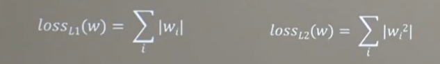
类型：正则化有两种类型：

一种是所有参数值的和（注意：正则化不会惩罚偏置ｂ，即只有ｗ被惩罚）的绝对值乘以惩罚权重，另外一种时所有参数的平方和乘以权重。

一般而言，正则化权重REGULARIZER = 0.03

我们用例子来直观感受正则化的作用

我们将用一个简单的数据集对坐标平面的点分类

数据集：

没有正则化的情况：

import tensorflow as tf
from matplotlib import pyplot as plt
import numpy as np
import pandas as pd
# 读入数据/标签 生成x_train y_train
df = pd.read_csv('dot.csv')
x_data = np.array(df[['x1', 'x2']])
y_data = np.array(df['y_c'])
x_train = np.vstack(x_data).reshape(-1, 2)
y_train = np.vstack(y_data).reshape(-1, 1)
Y_c = [['red' if y else 'blue'] for y in y_train]
# 转换x的数据类型，否则后面矩阵相乘时会因数据类型问题报错
x_train = tf.cast(x_train, tf.float32)
y_train = tf.cast(y_train, tf.float32)
# from_tensor_slices函数切分传入的张量的第一个维度，生成相应的数据集，使输入特征和标签值一一对应
train_db = tf.data.Dataset.from_tensor_slices((x_train, y_train)).batch(32)
# 生成神经网络的参数，输入层为2个神经元，隐藏层为11个神经元，1层隐藏层，输出层为1个神经元
# 用tf.Variable()保证参数可训练
w1 = tf.Variable(tf.random.normal([2, 11]), dtype=tf.float32)
b1 = tf.Variable(tf.constant(0.01, shape=[11]))
w2 = tf.Variable(tf.random.normal([11, 1]), dtype=tf.float32)
b2 = tf.Variable(tf.constant(0.01, shape=[1]))
lr = 0.005  # 学习率
epoch = 800  # 循环轮数
# 训练部分
for epoch in range(epoch):
    for step, (x_train, y_train) in enumerate(train_db):
        with tf.GradientTape() as tape:  # 记录梯度信息
            h1 = tf.matmul(x_train, w1) + b1  # 记录神经网络乘加运算
            h1 = tf.nn.relu(h1)
            y = tf.matmul(h1, w2) + b2
            # 采用均方误差损失函数mse = mean(sum(y-out)^2)
            loss = tf.reduce_mean(tf.square(y_train - y))
        # 计算loss对各个参数的梯度
        variables = [w1, b1, w2, b2]
        grads = tape.gradient(loss, variables)
        # 实现梯度更新
        # w1 = w1 - lr * w1_grad tape.gradient是自动求导结果与[w1, b1, w2, b2] 索引为0，1，2，3
        w1.assign_sub(lr * grads[0])
        b1.assign_sub(lr * grads[1])
        w2.assign_sub(lr * grads[2])
        b2.assign_sub(lr * grads[3])
    # 每20个epoch，打印loss信息
    if epoch % 20 == 0:
        print('epoch:', epoch, 'loss:', float(loss))
# 预测部分
print("*******predict*******")
# xx在-3到3之间以步长为0.01，yy在-3到3之间以步长0.01,生成间隔数值点
xx, yy = np.mgrid[-3:3:.1, -3:3:.1]
# 将xx , yy拉直，并合并配对为二维张量，生成二维坐标点
grid = np.c_[xx.ravel(), yy.ravel()]
grid = tf.cast(grid, tf.float32)
# 将网格坐标点喂入神经网络，进行预测，probs为输出
probs = []
for x_test in grid:
    # 使用训练好的参数进行预测
    h1 = tf.matmul([x_test], w1) + b1
    h1 = tf.nn.relu(h1)
    y = tf.matmul(h1, w2) + b2  # y为预测结果
    probs.append(y)
# 取第0列给x1，取第1列给x2
x1 = x_data[:, 0]
x2 = x_data[:, 1]
# probs的shape调整成xx的样子
probs = np.array(probs).reshape(xx.shape)
plt.scatter(x1, x2, color=np.squeeze(Y_c))  # squeeze去掉纬度是1的纬度,相当于去掉[['red'],[''blue]],内层括号变为['red','blue']
# 把坐标xx yy和对应的值probs放入contour函数，给probs值为0.5的所有点上色  plt.show()后 显示的是红蓝点的分界线
plt.contour(xx, yy, probs, levels=[.5])
plt.show()
# 读入红蓝点，画出分割线，不包含正则化
# 不清楚的数据，建议print出来查看

结果：

有正则化的情况：

# 正则化：一班只对w使用而不对偏置b使用
# 正则化的惩罚项可以是所有w的绝对值求和（稀疏参数使部分参数为零）以及平方求和（减小参数大小但不为零）再乘以权重
# 导入所需模块
import tensorflow as tf
from matplotlib import pyplot as plt
import numpy as np
import pandas as pd

# 读入数据/标签 生成x_train y_train
df = pd.read_csv('dot.csv')
x_data = np.array(df[['x1', 'x2']])
y_data = np.array(df['y_c'])
x_train = x_data
# 用reshape函数改变array的形状，改为一列
y_train = y_data.reshape(-1, 1)
# print(y_data)
# print(y_train)
Y_c = [['red' if y else 'blue'] for y in y_train]
# 转换x的数据类型，否则后面矩阵相乘时会因数据类型问题报错
x_train = tf.cast(x_train, tf.float32)
y_train = tf.cast(y_train, tf.float32)
# from_tensor_slices函数切分传入的张量的第一个维度，生成相应的数据集，使输入特征和标签值一一对应
train_db = tf.data.Dataset.from_tensor_slices((x_train, y_train)).batch(32)
# 生成神经网络的参数，输入层为4个神经元，隐藏层为32个神经元，2层隐藏层，输出层为3个神经元
# 用tf.Variable()保证参数可训练
w1 = tf.Variable(tf.random.normal([2, 11]), dtype=tf.float32)
b1 = tf.Variable(tf.constant(0.01, shape=[11]))
w2 = tf.Variable(tf.random.normal([11, 1]), dtype=tf.float32)
b2 = tf.Variable(tf.constant(0.01, shape=[1]))
lr = 0.005  # 学习率为
epoch = 800  # 循环轮数
# 训练部分
for epoch in range(epoch):
    for step, (x_train, y_train) in enumerate(train_db):
        with tf.GradientTape() as tape:  # 记录梯度信息
            h1 = tf.matmul(x_train, w1) + b1  # 记录神经网络乘加运算
            h1 = tf.nn.relu(h1)
            y = tf.matmul(h1, w2) + b2
            # 采用均方误差损失函数mse = mean(sum(y-out)^2)
            loss_mse = tf.reduce_mean(tf.square(y_train - y))
            # 添加l2正则化
            loss_regularization = []
            # tf.nn.l2_loss(w)=sum(w ** 2) / 2
            loss_regularization.append(tf.nn.l2_loss(w1))
            loss_regularization.append(tf.nn.l2_loss(w2))
            # 求和
            # 例：x=tf.constant(([1,1,1],[1,1,1]))
            #   tf.reduce_sum(x)
            # >>>6
            loss_regularization = tf.reduce_sum(loss_regularization)
            loss = loss_mse + 0.03 * loss_regularization  # REGULARIZER = 0.03
        # 计算loss对各个参数的梯度
        variables = [w1, b1, w2, b2]
        grads = tape.gradient(loss, variables)
        # 实现梯度更新
        # w1 = w1 - lr * w1_grad
        w1.assign_sub(lr * grads[0])
        b1.assign_sub(lr * grads[1])
        w2.assign_sub(lr * grads[2])
        b2.assign_sub(lr * grads[3])
    # # 每200个epoch，打印loss信息
    # if epoch % 20 == 0:
    #     print('epoch:', epoch, 'loss:', float(loss))
# 预测部分
print("*******predict*******")
# xx在-3到3之间以步长为0.01，yy在-3到3之间以步长0.1,生成间隔数值点
xx, yy = np.mgrid[-3:3:.1, -3:3:.1]
# print(xx)
# print(yy)
# 将xx, yy拉直，并合并配对为二维张量，生成二维坐标点
grid = np.c_[xx.ravel(), yy.ravel()]
# print(grid)
grid = tf.cast(grid, tf.float32)
# 将网格坐标点喂入神经网络，进行预测，probs为输出
probs = []
for x_predict in grid:
    # 使用训练好的参数进行预测
    # 低维和高维数据相加，会转化为高维数据，而仅同为数据才可以做矩阵乘法
    h1 = tf.matmul([x_predict], w1) + b1
    # print(h1)
    h1 = tf.nn.relu(h1)
    y = tf.matmul(h1, w2) + b2  # y为预测结果
    # print(y)
    probs.append(y)
# 取第0列给x1，取第1列给x2
x1 = x_data[:, 0]
x2 = x_data[:, 1]
# probs的shape调整成xx的样子,并且将张量转化为了array
# print(probs)
probs = np.array(probs).reshape(xx.shape)
# print(probs)
# print(Y_c)
plt.scatter(x1, x2, color=np.squeeze(Y_c))
# 把坐标xx yy和对应的值probs放入contour函数，给probs值为0.5的所有点上色  plt.show()后 显示的是红蓝点的分界线
plt.contour(xx, yy, probs, levels=[.5])
plt.show()
# # 读入红蓝点，画出分割线，包含正则化
# # 不清楚的数据，建议print出来查看

结果：

总结：通过以上的例子，我们可以看出正则化过后的分界线更加平滑，没有正则化的分类能明显有过拟合的嫌疑，正则化通常可以很好的增加模型的准确性，在实际中获得更好的表现。

链接：

https://www.icourse163.org/learn/PKU-1002536002?tid=1452937471#/learn/content?type=detail&id=1229845557&cid=1247337355&replay=true

甘霖那

关注

0
点赞
踩
0

收藏

觉得还不错? 一键收藏
0
评论
过拟合和欠拟合问题

一、介绍关于过拟合和欠拟合问题产生的原因及其后果，这类文章已经很多，那如何解决该问题？常用以下方法：# 欠拟合：增加输入项特征、增加网络参数、减少正则化参数# 过拟合：数据清洗、增大数据集、正则化、增大正则化参数二、正则化的作用原理：正则化通过加入惩罚项控制参数的大小不会剧烈变化，从而使预测曲线更加平滑组成：加入正则化的损失函数包含两部分，一部分是原来的损失函数，另一部分是惩罚项：类...
复制链接

扫一扫