决策树算法原理详解+python代码实现

决策树算法原理详解+python代码实现

一、原理分析

决策树算法的一般步骤：

1. 数据准备： 收集并准备带有标签的训练数据。
2. 特征选择： 选择对于问题有意义的特征作为节点进行决策。
3. 树的生成： 通过递归地将数据集划分为子集，建立决策树。常见的划分策略有信息熵、基尼系数等。
4. 树的修剪： 为了防止过拟合，可以对生成的树进行剪枝。
5. 预测： 使用生成的决策树进行新数据的分类或回归预测。

1.1 计算信息熵

定义： 熵度量的随机变量的不确定性，信息熵越大，从而样本纯度越低。ID3算法的核心思想是以信息增益来度量特征选择，选择信息增益最大的特征进行决策。算法采用自顶向下的贪婪搜索遍历可能的决策树空间。

设 $X$ 是一个取有限个值的离散随机变量，其概率分布为

$$P(X=x_i)=p_i$$

则随机变量 $X$ 的熵定义为

$$H(X)=-\sum _{i=1}^n{p}_i\log p_i$$

其中 $p_i=0$ 时，$0\log 0=0$。通常对数以2或 $e$ 为底，则熵的单位为比特（bit）或纳特(nat)。熵只依赖于 $X$ 的分布，而与 $X$ 的取值无关，所以 $H(x)$ 也记作 $H(p)$。

$$0\le H(p)\le \log n$$

方法步骤： 创建数据字典，键值为最后一列的数值，每个键值都记录了当前类别出现的次数。 使用所有类别的发生频率计算类别出现概率。

1.2 计算基尼系数

定义： 基尼系数是一种衡量数据集纯度（impurity）的指标，通常用于决策树算法中。对于一个给定的数据集，基尼系数越小，表示数据集的纯度越高，也就是说数据集中的样本越趋向于属于同一类别。

基尼系数的计算方式如下：

$textGini=1-{\sum }_{i=1}^c{p}_i^2$

其中，(c)是类别的数量，$p_i$是数据集中属于第 (i) 个类别的样本占比。基尼系数的取值范围是 0 到 1，取 0 表示数据集完全纯净，即所有样本属于同一类别；取 1 表示数据集的混合度最高，即各类别样本均匀分布。

1.3 针对每个特征，计算信息增益或基尼减小量：

对于每个特征，算法计算其划分数据集后的信息增益或基尼减小量。

• 信息增益：
  $\text{Information Gain}={\text{Entropy}}_{\text{before}}-{\sum }_j\frac{|S_j|}{|S|}\times {\text{Entropy}}_{\text{after}}(S_j)$
  这里，$|S|$是节点样本总数，$|S_j|$是特征划分后第(j)个子集的样本数，${\text{Entropy}}_{\text{before}}$和${\text{Entropy}}_{\text{after}}(S_j)$分别是划分前和划分后的节点熵。

• 基尼减小量：
  $\text{Gini Decrease}={\text{Gini}}_{\text{before}}-{\sum }_j\frac{|S_j|}{|S|}\times {\text{Gini}}_{\text{after}}(S_j)$
  其中，${\text{Gini}}_{\text{before}}$和${\text{Gini}}_{\text{after}}(S_j)$分别是划分前和划分后的节点基尼系数。

二、从零实现决策树算法

2.1 决策树的构造

​ 决策树是一个非常常见且优秀的机器学习算法，它易于理解、可解释性强，其可作为分类算法，也可用于回归模型。基本树的算法有ID3算法、C4.5算法、和CART算法。本次实验中，我们采用ID3算法构建。

1. 初始化特征集合和数据集合；
2. 计算数据集合信息熵和所有特征的条件熵，选择信息增益最大的特征作为当前决策节点；
3. 更新数据集合和特征集合（删除上一步使用的特征，并按照特征值来划分不同分支的数据集合）；
4. 重复 2，3 两步，若子集值包含单一特征，则为分支叶子节点。

决策树由节点和有向边组成。节点有两种类型：内部节点和叶节点。内部节点表示一个特征或属性，叶节点表示一个类。

用决策树进行分类，从根节点开始，对实例的某一个特征进行测试，根据测试结果，将实例分配到其子节点；如此递归地对实例进行测试并分配，直至到达叶节点。

• 导入数据集

def createDataSet():
    dataSet = [[1, 1, 'yes'],
               [1, 1, 'yes'],
               [1, 0, 'no'],
               [0, 1, 'no'],
               [0, 1, 'no']]
    labels = ['no surfacing', 'flippers']
    #change to discrete values
    return dataSet, labels
mydat,labels=createDataSet()

mydat：[[1, 1, ‘yes’], [1, 1, ‘yes’], [1, 0, ‘no’], [0, 1, ‘no’], [0, 1, ‘no’]]

labels：[‘no surfacing’, ‘flippers’]

• 计算数据集的信息熵

from math import log
def calcShannonEnt(dataSet):
    numEntries = len(dataSet)
    labelCounts = {}
    for featVec in dataSet: #the the number of unique elements and their occurance
        currentLabel = featVec[-1]
        if currentLabel not in labelCounts.keys(): labelCounts[currentLabel] = 0
        labelCounts[currentLabel] += 1
    shannonEnt = 0.0
    for key in labelCounts:
        prob = float(labelCounts[key])/numEntries
        shannonEnt -= prob * log(prob, 2) #log base 2
    return shannonEnt
calcShannonEnt(mydat)

0.9709505944546686

2.1.1 划分数据集

​ ID3 算法使用的分类标准是信息增益，它表示得知特征 A 的信息而使得样本集合不确定性减少的程度。对每一个特征划分数据集的结果计算一次信息熵，然后判断那个特征划分数据集的结果最好。 当我们按照某个特征划分数据集的时候，就需要将所有符合要求的元素抽取出来。 根据计算的熵值判断最好的划分方式。

**信息增益：**信息增益 $g(D,A)$ 表示得知特征 $X$ 的信息，而使类的信息 $Y$ 的不确定性减少的程度。信息增益大的特征分类能力强。

$$g(D,A)=H(D)-H(D|A)$$

$$H(D)=-\sum _{k=1}^K\frac{\left|C_k\right|}{|D|}{\log }_2\frac{\left|C_k\right|}{|D|}$$

$$H(D|A)=\sum _{i=1}^n\frac{\left|D_i\right|}{|D|}H(D_i)=-\sum _{i=1}^n\frac{\left|D_i\right|}{|D|}\sum _{k=1}^K\frac{\left|D_{ik}\right|}{\left|D_i\right|}{\log }_2\frac{\left|D_{ik}\right|}{\left|D_i\right|}$$

其中，$\left|C_k\right|$ 为类 $C_k$ 的样本个数，$|D|$ 表示样本容量。特征 $A$ 有 $n$ 个不同的取值 { a 1 , a 2 , ⋯   , a n } \{a_1, a_2, \cdots, a_n\} {a1​,a2​,⋯,an​}，根据取值将 $D$ 划分为 $n$ 个子集 $D_1,D_2,\cdots ,D_n$，$\left|D_i\right|$ 为 $D_i$ 的样本个数。$D_{ik}=D_i\cap C_k$。

• 按照给定特征划分数据集

def splitDataSet(dataSet, axis, value):
    retDataSet = []
    for featVec in dataSet:
        if featVec[axis] == value:
            reducedFeatVec = featVec[:axis]     #chop out axis used for splitting
            reducedFeatVec.extend(featVec[axis+1:])
            retDataSet.append(reducedFeatVec)
    return retDataSet

• 选择最好的划分方式

def chooseBestFeatureToSplit(dataSet):
    numFeatures = len(dataSet[0]) - 1      #the last column is used for the labels
    baseEntropy = calcShannonEnt(dataSet)   #计算整个数据集的原始信息熵
    bestInfoGain = 0.0; bestFeature = -1
    for i in range(numFeatures):        #iterate over all the features
        featList = [example[i] for example in dataSet]#create a list of all the examples of this feature
        uniqueVals = set(featList)       #get a set of unique values
        newEntropy = 0.0
        for value in uniqueVals:
            subDataSet = splitDataSet(dataSet, i, value)
            prob = len(subDataSet)/float(len(dataSet))
            newEntropy += prob * calcShannonEnt(subDataSet)
        infoGain = baseEntropy - newEntropy     #calculate the info gain; ie reduction in entropy
        if (infoGain > bestInfoGain):       #compare this to the best gain so far
            bestInfoGain = infoGain         #if better than current best, set to best
            bestFeature = i
    return bestFeature                      #returns an integer

2.1.2 递归构建决策树

​ 根据原始数据集，基于最好的属性值划分数据集，由于特征值可能有多个，因此可能存在大于两个分支的数据集划分。第一次划分之后，数据将被向下传递到树分支的下一个节点，在这个点上，我们可以进一步划分数据集。采用递归的原则处理数据集。当划分完所有的属性，或者每个分支下的所有实例都具有相同的分类时，跳出递归循环。

• 采用多数表决的方法决定该叶子节点的分类

def majorityCnt(classList):
    classCount={}
    for vote in classList:
        if vote not in classCount.keys(): classCount[vote] = 0
        classCount[vote] += 1
    sortedClassCount = sorted(classCount.items(), key=operator.itemgetter(1), reverse=True)
    return sortedClassCount[0][0]

• 创建数的函数代码

def createTree(dataSet, labels):
    classList = [example[-1] for example in dataSet]
    if classList.count(classList[0]) == len(classList):
        return classList[0]#stop splitting when all of the classes are equal
    if len(dataSet[0]) == 1: #stop splitting when there are no more features in dataSet
        return majorityCnt(classList)
    bestFeat = chooseBestFeatureToSplit(dataSet)
    bestFeatLabel = labels[bestFeat]
    myTree = {bestFeatLabel:{}}
    del(labels[bestFeat])
    featValues = [example[bestFeat] for example in dataSet]
    uniqueVals = set(featValues)
    for value in uniqueVals:
        subLabels = labels[:]       #copy all of labels, so trees don't mess up existing labels
        myTree[bestFeatLabel][value] = createTree(splitDataSet(dataSet, bestFeat, value), subLabels)
    return myTree
createTree(mydat, labels)

{‘no surfacing’: {0: ‘no’, 1: {‘flippers’: {0: ‘no’, 1: ‘yes’}}}}

2.2 用Matplotlib绘制树形图

2.2.1 Matplotlib 注解

​ 使用Matplotlib提供的注解工具annotations,它可以在数据图形上添加文本注释。并且可以对文字着色并提供多种形状以供选择，且可以反转箭头，使箭头指向数据框。Matplotlib实际上是一套面向对象的绘图库，它所绘制的图表中的每个绘图元素，例如线条Line2D、文字Text、刻度等在内存中都有一个对象与之对应。

• 使用文本注解绘制节点

import matplotlib.pyplot as plt  # 载入 pyplot API
decisionNode = dict(boxstyle="sawtooth", fc="0.8") # 注（a）
leafNode = dict(boxstyle="round4", "fc=0.8")
arrow_args = dict(arrowstyle="<-")  # 箭头样式

def plotNode(Nodename, centerPt, parentPt, nodeType):  #  centerPt节点中心坐标  parentPt 起点坐标
    creatPlot.ax1.annotate(Nodename, xy=parentPt, xycoords='axes fraction', xttest=centerPt, textcoords='axes fraction', va="center", ha="center", bbox=nodeType, arrowprops=arrow_args) # 注（b）

def creatplot():
    fig = plt.figure(1, facecolor='white') # 创建一个新图形
    fig.clf() #  清空绘图区
    creatplot.ax1 = plt.subplot(111,frameon=False)  # subplot(323)和subplot(3,2,3)是相同的
    plotNode('decision Node', (0.5,0.1), (0.1,0.5), decisionNode)
    plotNode('leaf Node', (0.8,0.1), (0.3,0.8), leafNode)
    plt.show()
createPlot()

• 构造注解树

构造函数getNumleafs()和函数getTreeDepth()获取树的叶节点数目和树的层数。

def getNumLeafs(myTree):
    numLeafs = 0
    firstStr = list(myTree)[0]
    secondDict = myTree[firstStr]
    for key in secondDict.keys():
        if type(secondDict[key]).__name__ == 'dict':
            #test to see if the nodes are dictonaires, if not they are leaf nodes
#             type()函数用于判断子节点是否为字典类型
            numLeafs += getNumLeafs(secondDict[key])
        else: numLeafs += 1
    return numLeafs

def getTreeDepth(myTree):
    maxDepth = 0
    firstStr = list(myTree)[0]
    secondDict = myTree[firstStr]
    for key in secondDict.keys():
        if type(secondDict[key]).__name__ == 'dict':#test to see if the nodes are dictonaires, if not they are leaf nodes
            thisDepth = 1 + getTreeDepth(secondDict[key])
        else: thisDepth = 1
        if thisDepth > maxDepth: maxDepth = thisDepth
    return maxDepth

构造函数retrieveTree()输出预先存储的树信息，从而避免每次测试代码是都需要从数据中创建数的麻烦

def retrieveTree(i):
    listOfTrees = [{'no surfacing': {0: 'no', 1: {'flippers': {0: 'no', 1: 'yes'}}}},
                   {'no surfacing': {0: 'no', 1: {'flippers': {0: {'head': {0: 'no', 1: 'yes'}}, 1: 'no'}}}}
                  ]
    return listOfTrees[i]

2.2.2 plotTree()函数

​ 函数creatPlot()是我们使用的主函数，它调用了plotTree()，该函数首先计算树的宽度和高，全局变量plotTree.totalw存储树的宽度，全局变量plotTree.totalD存储树的深度，我们使用这两个变量计算树节点的摆放位置–使得树绘制在水平方向和垂直方向的中心位置。 进一步采用递归的思想，变量plotTree.XOff和plotTree.yOff追踪已经绘制的节点位置，以及放置下一节点的恰当位置。 接着，绘出子节点具有的特征值，使用函数plotMidText()计算父节点和子节点的中间位置，并天剑简单的文本标签。 由于我们是自顶向下绘制图形，所以需要按比例减少y坐标值，然后进一步递归。直至节点为叶子节点，则绘制出该节点。

def plotMidText(cntrPt, parentPt, txtString):
    xMid = (parentPt[0]-cntrPt[0])/2.0 + cntrPt[0]
    yMid = (parentPt[1]-cntrPt[1])/2.0 + cntrPt[1]
    createPlot.ax1.text(xMid, yMid, txtString, va="center", ha="center", rotation=30)

def plotTree(myTree, parentPt, nodeTxt):#if the first key tells you what feat was split on
    numLeafs = getNumLeafs(myTree)  #this determines the x width of this tree
    depth = getTreeDepth(myTree)
    firstStr = list(myTree)[0]     #the text label for this node should be this
    cntrPt = (plotTree.xOff + (1.0 + float(numLeafs))/2.0/plotTree.totalW, plotTree.yOff)
    plotMidText(cntrPt, parentPt, nodeTxt)
    plotNode(firstStr, cntrPt, parentPt, decisionNode)
    secondDict = myTree[firstStr]
    plotTree.yOff = plotTree.yOff - 1.0/plotTree.totalD
    for key in secondDict.keys():
        if type(secondDict[key]).__name__ == 'dict':#test to see if the nodes are dictonaires, if not they are leaf nodes
            plotTree(secondDict[key], cntrPt, str(key))        #recursion
        else:   #it's a leaf node print the leaf node
            plotTree.xOff = plotTree.xOff + 1.0/plotTree.totalW
            plotNode(secondDict[key], (plotTree.xOff, plotTree.yOff), cntrPt, leafNode)
            plotMidText((plotTree.xOff, plotTree.yOff), cntrPt, str(key))
    plotTree.yOff = plotTree.yOff + 1.0/plotTree.totalD
#if you do get a dictonary you know it's a tree, and the first element will be another dict

def createPlot02(inTree):
    fig = plt.figure(1, facecolor='white')
    fig.clf()
    axprops = dict(xticks=[], yticks=[])
    createPlot.ax1 = plt.subplot(111, frameon=False, **axprops)    #no ticks
    #createPlot.ax1 = plt.subplot(111, frameon=False) #ticks for demo puropses
    plotTree.totalW = float(getNumLeafs(inTree))
    plotTree.totalD = float(getTreeDepth(inTree))
    plotTree.xOff = -0.5/plotTree.totalW; plotTree.yOff = 1.0
    plotTree(inTree, (0.5, 1.0), '')
    plt.show()

myTree=retrieveTree(0) createPlot02(myTree)

myTree['no surfacing'][3]='maybe'
createPlot02(myTree)

2.3 测试和存储分类器

2.3.1 测试算法：使用决策树执行分类

​ 依靠训练数据构造决策树后，我们可以将其运用于实际数据的分类，在执行是需要使用决策树以及用于构造决策树的标签向量。比较测试数据与决策树上的数值。

• 使用决策树的分类函数

def classify(inputTree, featLabels, testVec):
    firstStr = list(inputTree)[0]
    secondDict = inputTree[firstStr]
    featIndex = featLabels.index(firstStr)
    key = testVec[featIndex]
#     将标签字符串转换为索引
    valueOfFeat = secondDict[key]
    if isinstance(valueOfFeat, dict):
        classLabel = classify(valueOfFeat, featLabels, testVec)
    else: classLabel = valueOfFeat
    return classLabel

第二节点为flippers，1叶子节点的类标签为yes

classify(myTree, labels, [1,1])

‘yes’

2.3.2 使用算法：决策树的存储

​ 决策树的构造十分耗时，为了节省时间，需要使用Python模块pickle序列化对象，序列化对象可以在磁盘上保存对象，并在需要的时候取出来。这样，就能在每次执行分类时调用已经构造好的决策树。

def storeTree(inputTree, filename):
    import pickle
    fw = open(filename, 'wb')
    pickle.dump(inputTree, fw)
    fw.close()

def grabTree(filename):
    import pickle
    fr = open(filename, 'rb')
    return pickle.load(fr)
storeTree(myTree, 'classifierStorage.txt')
grabTree('classifierStorage.txt')

2.4 实例：使用决策树预测隐形眼镜类型

(1)收集数据：提供的文本文件

(2)准备数据：解析tab键分隔的数据行

(3)分析数据：快速检查数据，确保正确地解析数据内容，使用ceatePlot()函数绘制树形图

(4)训练算法：creatTree()函数

(5)测试算法：编写测试函数验证决策时可以正确分类给定的数据实例

(6)使用算法：存储树的数据结构，以便下次使用时可以直接调用

import operator
fr=open('lenses.txt')
lenses=[inst.strip().split('\t') for inst in fr.readlines()]
lensesLabels=['age','prescript','astigmatic','tearRate']
lensesTree=createTree(lenses,lensesLabels)
lensesTree

{‘tearRate’: {‘normal’: {‘astigmatic’: {‘no’: {‘age’: {‘pre’: ‘soft’,
‘presbyopic’: {‘prescript’: {‘hyper’: ‘soft’, ‘myope’: ‘no lenses’}},
‘young’: ‘soft’}},
‘yes’: {‘prescript’: {‘hyper’: {‘age’: {‘pre’: ‘no lenses’,
‘presbyopic’: ‘no lenses’,
‘young’: ‘hard’}},
‘myope’: ‘hard’}}}},
‘reduced’: ‘no lenses’}}

createPlot02(lensesTree)

训练结果：沿着决策树的不同分支，我们可以得到不同患者需要佩戴的隐形眼镜类型。从图中我们可以知道，医生最多需要问四个问题就能患者需要佩戴哪种类型的隐形眼镜。

2.5 实验改进

上述实例中非常完美地匹配了实验数据，可能存在过拟合overfitting，考虑使用决策树剪枝算法降低拟合度，提高实际分类时的精度。

其次，对于数据集的处理也可能存在一些问题。

• 改进：采用交叉验证训练数据

import numpy as np
lenses2=np.array(lenses)
lenses2[::,4]
len(lenses2[::,4])

from sklearn.model_selection import train_test_split
from sklearn.metrics import accuracy_score
from sklearn import tree
# 避免过拟合，采用交叉验证，随机选取33%数据作为测试集，剩余为训练集
train_features, test_features, train_labels, test_labels = train_test_split(lenses, lenses2[::,4], test_size=0.33, random_state=0)

lensesLabels=['age','prescript','astigmatic','tearRate']
lensesTree=createTree(train_features,lensesLabels)
lensesTree
createPlot02(lensesTree)

lensesLabels=['age','prescript','astigmatic','tearRate']
j=0
for i in range(len(test_features)):
    test_predict = classify(lensesTree,lensesLabels,test_features[i])
    if test_predict == None:
        test_predict = epsilon
    if test_labels[i]==test_predict:
            j=j+1
score = j/i
print("The accruacy score is %f" % score)

The accruacy score is 0.857143
准确率为0.857 预测效果较好

三、机器学习实现决策树算法

# 导入必要的库
from sklearn.datasets import load_iris
from sklearn.model_selection import train_test_split
from sklearn.tree import DecisionTreeClassifier
from sklearn.metrics import accuracy_score

# 加载鸢尾花数据集
iris = load_iris()
X = iris.data
y = iris.target

# 将数据集划分为训练集和测试集
X_train, X_test, y_train, y_test = train_test_split(X, y, test_size=0.2, random_state=42)

# 创建决策树模型
model = DecisionTreeClassifier()

# 在训练集上训练模型
model.fit(X_train, y_train)

# 在测试集上进行预测
y_pred = model.predict(X_test)

# 计算模型的准确性
accuracy = accuracy_score(y_test, y_pred)
print(f"模型的准确性：{accuracy}")

# 使用训练好的模型进行新数据点的预测
new_data_point = [[5.1, 3.5, 1.4, 0.2]]
prediction = model.predict(new_data_point)
print(f"新数据点的预测结果：{prediction}")

模型的准确性：1.0
新数据点的预测结果：[0]

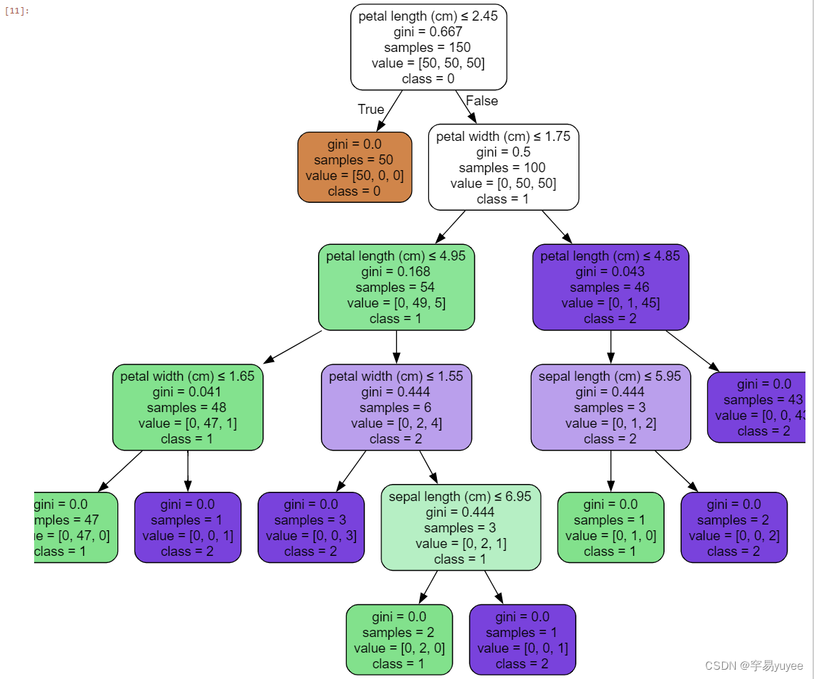
使用 Graphviz 工具进行决策树可视化

需要安装 Graphviz 软件和 graphviz Python 包

https://graphviz.org/

pip install graphviz

labels=['sepal length (cm)',
  'sepal width (cm)',
  'petal length (cm)',
  'petal width (cm)']


from sklearn.tree import DecisionTreeClassifier, export_graphviz
import os   
from sklearn import tree
import graphviz

os.environ["PATH"] += os.pathsep + 'C:/Program Files (x86)/Graphviz/Graphviz-10.0.1-win64/bin/' #路径名称根据你的路径进行替换

target=y
clf = tree.DecisionTreeClassifier()
clf = clf.fit(X,y)

dot_data = tree.export_graphviz(clf, out_file=None) 
graph = graphviz.Source(dot_data) 
graph.render("鸢尾花分类问题") 
target_name=['0','1','2']

dot_data = tree.export_graphviz(clf, out_file=None, 
                         feature_names=labels,  
                         class_names=target_name,  
                         filled=True, rounded=True,  
                         special_characters=True)  

graph = graphviz.Source(dot_data)
graph