


Multi-View Mesh Reconstruction with Neural Deferred Shading
1、Introduction
-
point-nerf和mobile-nerf和这篇都把mesh(geometry)和mlp联合优化。
-
Problem: While fully neural approaches are general, both in terms of geometry and appearance, current methods exhibit excessive runtime, making them impractical for domains that handle a large number of objects or multi-view video (e.g. of human performances).
-
We propose Neural Deferred Shading (NDS), a fast analysis-by-synthesis method that combines triangle meshes and neural rendering. The rendering pipeline is inspired by real-time graphics and implements a technique called deferred shading: a triangle mesh is first rasterized and the pixels are then processed by a neural shader that models the interaction of geometry, material, and light. Since the rendering pipeline, including rasterization and shading, is differentiable, we can optimize the neural shader and the surface mesh with gradient descent . The explicit geometry representation enables fast convergence while the neural shader maintains the generality of the modeled appearance.
2、Method
Given a set of images I = { I 1 , ⋅ ⋅ ⋅ , I n } I = \{I_1, · · · , I_n\} I={I1,⋅⋅⋅,In} from calibrated cameras and corresponding masks M = { M 1 , ⋅ ⋅ ⋅ , M n } M = \{M_1, · · · , M_n\} M={M1,⋅⋅⋅,Mn}, we want to estimate the 3D surface of an object shown in the images. To this end, we follow an analysis-by-synthesis approach: we find a surface that reproduces the images when rendered from the camera views. In this work, the surface is represented by a triangle mesh G = ( V , E , F ) G = (V, E, F) G=(V,E,F), consisting of vertex positions V , a set of edges E, and a set of faces F. We solve the optimization problem using gradient descent and gradually deform a mesh based on an objective function that compares renderings of the mesh to the input images.
![[外链图片转存失败,源站可能有防盗链机制,建议将图片保存下来直接上传(img-uEmkQ447-1661506026965)(C:\Users\47008\AppData\Roaming\Typora\typora-user-images\image-20220808194739207.png)]](https://img-blog.csdnimg.cn/c22d238dc88d4306b652c5c24fe9aed3.png)
2.1. Neural Deferred Shading
![[外链图片转存失败,源站可能有防盗链机制,建议将图片保存下来直接上传(img-2YqPKYCw-1661506026966)(C:\Users\47008\AppData\Roaming\Typora\typora-user-images\image-20220808194845592.png)]](https://img-blog.csdnimg.cn/8884208e5b9449a1a46f6c46cc59e040.png)
Given a camera i, the mesh is rasterized in a first pass, yielding a triangle index and barycentric coordinates per pixel. This information is used to interpolate both vertex positions and vertex normals, creating a geometry buffer (g-buffer) with per-pixel positions and normals. In a second pass, the g-buffer is processed by a learned shader with parameters θ \theta θ.
![[外链图片转存失败,源站可能有防盗链机制,建议将图片保存下来直接上传(img-80OGzGVA-1661506026967)(C:\Users\47008\AppData\Roaming\Typora\typora-user-images\image-20220808202534566.png)]](https://img-blog.csdnimg.cn/09dd0382cfe14cbb91840dcfae134083.png)
The shader returns an RGB color value for a given position x ∈ R 3 x ∈ R^3 x∈R3, normal n ∈ R 3 n ∈ R^3 n∈R3, and view direction ω o = c i − x ∥ c i − x ∥ ω_o = \frac{ci−x} {∥ci−x∥} ωo=∥ci−x∥ci−x, with c i ∈ R 3 c_i ∈ R^3 ci∈R3 the center of camera i. It is optimized together with the geometry.
In addition to a color image, the renderer also produces a mask that indicates if a pixel is covered by the mesh.
2.2. Objective Function
Finding an estimate of shape and appearance formally corresponds to solving the following minimization problem in our framework:
![[外链图片转存失败,源站可能有防盗链机制,建议将图片保存下来直接上传(img-8hrWDhbn-1661506026967)(C:\Users\47008\AppData\Roaming\Typora\typora-user-images\image-20220808210951145.png)]](https://img-blog.csdnimg.cn/9526db07f92544f598be61a99cbc97aa.png)
where L a p p e a r a n c e L_{appearance} Lappearance compares the rendered appearance of the estimated surface to the camera images and L g e o m e t r y L_{geometry} Lgeometry regularizes the mesh to avoid undesired vertex configurations.
2.2.1. Apperance
The appearance objective is composed of two terms:
![(img-50mfSjTV-1661506026968)(C:\Users\47008\AppData\Roaming\Typora\typora-user-images\image-20220808212350601.png)]](https://img-blog.csdnimg.cn/ca253dec43eb497cb0696048a63a64d5.png)
where the shading term:
![[外链图片转存失败,源站可能有防盗链机制,建议将图片保存下来直接上传(img-XI1Q9huJ-1661506026968)(C:\Users\47008\AppData\Roaming\Typora\typora-user-images\image-20220808212407535.png)]](https://img-blog.csdnimg.cn/7b289082476346e1a60990493a20fcf6.png)
ensures that the color images produced by the shader
I
i
~
\widetilde{I_i}
Ii
correspond to the input images and the silhouette term ensures that the rendered masks
M
i
~
\widetilde{M_i}
Mi
match the input masks for all views.
![[外链图片转存失败,源站可能有防盗链机制,建议将图片保存下来直接上传(img-bF7zq4Yx-1661506026969)(C:\Users\47008\AppData\Roaming\Typora\typora-user-images\image-20220808213735000.png)]](https://img-blog.csdnimg.cn/72211ce81fb646a2af8251a7c78c3a70.png)
Formally, the masks M i ~ \widetilde{M_i} Mi are functions of the geometry G G G and the parameters of camera i.
Separating the shading from the silhouette objective mainly has performance reasons: For a camera view i, the rasterization considers all pixels in the image, therefore computing the mask M i ~ \widetilde{M_i} Mi is cheap. However, shading is more involved and requires invoking the neural shader for all pixels after rasterization, which is an expensive operation. In practice, we only shade a subset of pixels inside the intersection of input and rendered masks while comparing the silhouette for all pixels.
2.2.2. Geometry Regularization
Naively moving the vertices unconstrained in each iteration quickly leads to undesirable meshes with degenerate triangles and self-intersections.We use a geometry regularization term that favors smooth solutions and is inspired by Luan et al. :
![[外链图片转存失败,源站可能有防盗链机制,建议将图片保存下来直接上传(img-7TOM6XxW-1661506026969)(C:\Users\47008\AppData\Roaming\Typora\typora-user-images\image-20220808214411565.png)]](https://img-blog.csdnimg.cn/2a84f697b9f949b4a4e135d3b98d7bd8.png)
Let V ∈ R n × 3 V ∈ R^{n×3} V∈Rn×3 be a matrix with vertex positions as rows, the Laplacian term is defined as:
![[外链图片转存失败,源站可能有防盗链机制,建议将图片保存下来直接上传(img-8Ku67TdC-1661506026970)(C:\Users\47008\AppData\Roaming\Typora\typora-user-images\image-20220808214501848.png)]](https://img-blog.csdnimg.cn/d00145866e3047d2a18d1664da67204f.png)
where
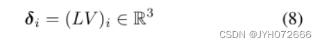
are the differential coordinates of vertex i, L ∈ R n × n L ∈ R^{n×n} L∈Rn×n is the graph Laplacian of the mesh G. Intuitively, by minimizing the magnitude of the differential coordinates of a vertex, we minimize its distance to the average position of its neighbors.
The normal consistency term is defined as:
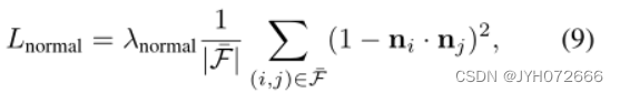
where F ‾ \overline{F} F is the set of triangle pairs that share an edge and n i ∈ R 3 n_i ∈ R^3 ni∈R3 is the normal of triangle i (under an arbitrary ordering of the triangles). It computes the cosine similarity between neighboring face normals and enforces additional smoothness.
2.3.3. Optimization
Our optimization starts from an initial mesh that is computed from the masks and resembles a visual hull. Alternatively, it can start from a custom mesh.


 2782
2782


 被折叠的 条评论
为什么被折叠?
被折叠的 条评论
为什么被折叠?
 到【灌水乐园】发言


