


坐标变换的艺术—高频注入法公式推导
PMSM无位置传感器技术总体而言可分为两个部分,第一部分获知位置误差信号然后输入位置观测器进行处理,使得位置信号收敛,第二部分是极性判断。本文着重讲解第一部分中位置误差信号的获取,至于后续的观测器、极性判断等环节,以及另外的感应电机的无速度传感器技术会在文末给出学习资料。
PMSM高频模型的由来
PMSM在旋转轴系的电压为
[
u
d
u
q
]
=
R
[
i
d
i
q
]
+
d
d
t
[
ψ
d
ψ
q
]
+
ω
e
[
−
ψ
q
ψ
d
]
(1)
\tag{1} \left[ \begin{array}{c} u_d\\ u_q\\ \end{array} \right] =R\left[ \begin{array}{c} i_d\\ i_q\\ \end{array} \right] +\frac{\mathrm{d}}{\mathrm{d}t}\left[ \begin{array}{c} \psi _d\\ \psi _q\\ \end{array} \right] +\omega _e\left[ \begin{array}{c} -\psi _q\\ \psi _d\\ \end{array} \right]
[uduq]=R[idiq]+dtd[ψdψq]+ωe[−ψqψd](1)
在零低速工况,基于一些假设,公式
(
1
)
(1)
(1)被进一步简化,习惯将简化后的方程称之为高频模型。通常,电机的电路模型视为R-L电路,控制回路中注入高频信号,此时电路中占据主导地位的是电感项,又因为电机运行于零低速,因此旋转电压方程中的第一项和第三项可忽略,则PMSM的高频电压模型为
[
u
d
h
u
q
h
]
=
d
d
t
[
ψ
d
ψ
q
]
=
[
L
d
0
0
L
q
]
d
d
t
[
i
d
h
i
q
h
]
(2)
\tag{2} \left[ \begin{array}{c} u_{dh}\\ u_{qh}\\ \end{array} \right] =\frac{\mathrm{d}}{\mathrm{d}t}\left[ \begin{array}{c} \psi _d\\ \psi _q\\ \end{array} \right] =\left[ \begin{matrix} L_d& 0\\ 0& L_q\\ \end{matrix} \right] \frac{\mathrm{d}}{\mathrm{d}t}\left[ \begin{array}{c} i_{dh}\\ i_{qh}\\ \end{array} \right]
[udhuqh]=dtd[ψdψq]=[Ld00Lq]dtd[idhiqh](2)
高频电压模型是高频注入法的核心所在,由此衍生出了旋转高频注入法、脉振高频注入法(脉振正弦和脉振方波)。
公式推导
为了便于公式推导,将式
(
2
)
(2)
(2)转换成电流微分表达式,可得:
d
d
t
[
i
d
h
i
q
h
]
=
[
1
L
d
0
0
1
L
q
]
[
u
d
h
u
q
h
]
(3)
\tag{3} \frac{\mathrm{d}}{\mathrm{d}t}\left[ \begin{array}{c} i_{dh}\\ i_{qh}\\ \end{array} \right] =\left[ \begin{matrix} \frac{1}{L_d}& 0\\ 0& \frac{1}{L_q}\\ \end{matrix} \right] \left[ \begin{array}{c} u_{dh}\\ u_{qh}\\ \end{array} \right]
dtd[idhiqh]=[Ld100Lq1][udhuqh](3)
所有的高频方波注入法遵循坐标变换理论,各坐标系间的关系如下图所示,
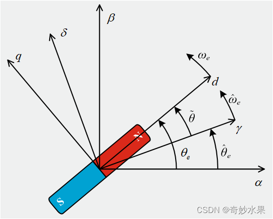
估计轴系至旋转轴系的坐标变换矩阵满足
P
γ
δ
/
d
q
=
[
cos
θ
~
sin
θ
~
−
sin
θ
~
cos
θ
~
]
(4)
\tag{4} P_{\gamma \delta /dq}=\left[ \begin{matrix} \cos \tilde{\theta}& \sin \tilde{\theta}\\ -\sin \tilde{\theta}& \cos \tilde{\theta}\\ \end{matrix} \right]
Pγδ/dq=[cosθ~−sinθ~sinθ~cosθ~](4)
静止轴系至旋转轴系的坐标变换矩阵满足
P α β / d q = [ cos θ e sin θ e − sin θ e cos θ e ] (5) \tag{5} P_{\alpha \beta /dq}=\left[ \begin{matrix} \cos \theta _e& \sin \theta _e\\ -\sin \theta _e& \cos \theta _e\\ \end{matrix} \right] Pαβ/dq=[cosθe−sinθesinθecosθe](5)
上述
(
4
)
(4)
(4)、
(
5
)
(5)
(5)是单位正交矩阵,满足
P
−
1
=
P
T
(6)
\tag{6} P^{-1}=P^T
P−1=PT(6)
为了读者更好的理解下文各高频注入法的公式推导过程,现将各方法的信号注入、响应信号提取轴系罗列成表,作为推导线索。
| 算法名称 | 高频电压信号注入轴系 | 高频电流提取轴系 |
|---|---|---|
| 旋转高频注入法 | 两相静止轴系 | 两相静止轴系 |
| 脉振高频正弦注入法 | 估计轴系 | 估计轴系 |
| 脉振高频方波注入法 | 估计轴系 | 静止轴系 |
旋转高频注入法
旋转高频注入法在静止轴系完成信号注入、响应信号提取过程,依据坐标变换理论,可得:
[
i
d
h
i
q
h
]
=
[
cos
θ
e
sin
θ
e
−
sin
θ
e
cos
θ
e
]
[
i
α
i
β
]
(7)
\tag{7} \left[ \begin{array}{c} i_{dh}\\ i_{qh}\\ \end{array} \right] =\left[ \begin{matrix} \cos \theta _e& \sin \theta _e\\ -\sin \theta _e& \cos \theta _e\\ \end{matrix} \right] \left[ \begin{array}{c} i_{\alpha}\\ i_{\beta}\\ \end{array} \right]
[idhiqh]=[cosθe−sinθesinθecosθe][iαiβ](7)
[ u d h u q h ] = [ cos θ e sin θ e − sin θ e cos θ e ] [ u α u β ] (8) \tag{8} \left[ \begin{array}{c} u_{dh}\\ u_{qh}\\ \end{array} \right] =\left[ \begin{matrix} \cos \theta _e& \sin \theta _e\\ -\sin \theta _e& \cos \theta _e\\ \end{matrix} \right] \left[ \begin{array}{c} u_{\alpha}\\ u_{\beta}\\ \end{array} \right] [udhuqh]=[cosθe−sinθesinθecosθe][uαuβ](8)
结合式
(
7
)
(7)
(7),对式
(
3
)
(3)
(3)中等式左边的微分项化简,可得:
d
d
t
[
i
d
h
i
q
h
]
=
d
d
t
{
[
cos
θ
e
sin
θ
e
−
sin
θ
e
cos
θ
e
]
[
i
α
i
β
]
}
=
[
−
sin
θ
e
cos
θ
e
−
cos
θ
e
−
sin
θ
e
]
ω
e
[
i
α
i
β
]
+
[
cos
θ
e
sin
θ
e
−
sin
θ
e
cos
θ
e
]
d
d
t
[
i
α
i
β
]
(9)
\tag{9} \frac{\mathrm{d}}{\mathrm{d}t}\left[ \begin{array}{c} i_{dh}\\ i_{qh}\\ \end{array} \right] =\frac{\mathrm{d}}{\mathrm{d}t}\left\{ \left[ \begin{matrix} \cos \theta _e& \sin \theta _e\\ -\sin \theta _e& \cos \theta _e\\ \end{matrix} \right] \left[ \begin{array}{c} i_{\alpha}\\ i_{\beta}\\ \end{array} \right] \right\} =\left[ \begin{matrix} -\sin \theta _e& \cos \theta _e\\ -\cos \theta _e& -\sin \theta _e\\ \end{matrix} \right] \omega _e\left[ \begin{array}{c} i_{\alpha}\\ i_{\beta}\\ \end{array} \right] +\left[ \begin{matrix} \cos \theta _e& \sin \theta _e\\ -\sin \theta _e& \cos \theta _e\\ \end{matrix} \right] \frac{\mathrm{d}}{\mathrm{d}t}\left[ \begin{array}{c} i_{\alpha}\\ i_{\beta}\\ \end{array} \right]
dtd[idhiqh]=dtd{[cosθe−sinθesinθecosθe][iαiβ]}=[−sinθe−cosθecosθe−sinθe]ωe[iαiβ]+[cosθe−sinθesinθecosθe]dtd[iαiβ](9)
分析式
(
9
)
(9)
(9),展开式中的第一项含有速度项,因电机运行于零低速工况,故第一项略去,保留第二项,可得:
d
d
t
[
i
d
h
i
q
h
]
=
[
cos
θ
e
sin
θ
e
−
sin
θ
e
cos
θ
e
]
d
d
t
[
i
α
i
β
]
(10)
\tag{10} \frac{\mathrm{d}}{\mathrm{d}t}\left[ \begin{array}{c} i_{dh}\\ i_{qh}\\ \end{array} \right] =\left[ \begin{matrix} \cos \theta _e& \sin \theta _e\\ -\sin \theta _e& \cos \theta _e\\ \end{matrix} \right] \frac{\mathrm{d}}{\mathrm{d}t}\left[ \begin{array}{c} i_{\alpha}\\ i_{\beta}\\ \end{array} \right]
dtd[idhiqh]=[cosθe−sinθesinθecosθe]dtd[iαiβ](10)
将
(
8
)
(8)
(8)、
(
10
)
(10)
(10)带入式
(
3
)
(3)
(3),结合式
(
6
)
(6)
(6),式
(
3
)
(3)
(3)可重写为
d
d
t
[
i
α
h
i
β
h
]
=
[
cos
θ
e
−
sin
θ
e
sin
θ
e
cos
θ
e
]
[
1
L
d
0
0
1
L
q
]
[
cos
θ
e
sin
θ
e
−
sin
θ
e
cos
θ
e
]
[
u
α
h
u
β
h
]
(11)
\tag{11} \frac{\mathrm{d}}{\mathrm{d}t}\left[ \begin{array}{c} i_{\alpha h}\\ i_{\beta h}\\ \end{array} \right] =\left[ \begin{matrix} \cos \theta _e& -\sin \theta _e\\ \sin \theta _e& \cos \theta _e\\ \end{matrix} \right] \left[ \begin{matrix} \frac{1}{L_d}& 0\\ 0& \frac{1}{L_q}\\ \end{matrix} \right] \left[ \begin{matrix} \cos \theta _e& \sin \theta _e\\ -\sin \theta _e& \cos \theta _e\\ \end{matrix} \right] \left[ \begin{array}{c} u_{\alpha h}\\ u_{\beta h}\\ \end{array} \right]
dtd[iαhiβh]=[cosθesinθe−sinθecosθe][Ld100Lq1][cosθe−sinθesinθecosθe][uαhuβh](11)
对式
(
11
)
(11)
(11)中等式右边的矩阵乘积因子化简,可得:
[
cos
θ
e
−
sin
θ
e
sin
θ
e
cos
θ
e
]
[
1
L
d
0
0
1
L
q
]
[
cos
θ
e
sin
θ
e
−
sin
θ
e
cos
θ
e
]
⇒
[
1
2
(
1
L
d
+
1
L
q
)
+
1
2
(
1
L
d
−
1
L
q
)
cos
2
θ
e
1
2
(
1
L
d
−
1
L
q
)
sin
2
θ
e
1
2
(
1
L
d
−
1
L
q
)
sin
2
θ
e
1
2
(
1
L
d
+
1
L
q
)
−
1
2
(
1
L
d
−
1
L
q
)
cos
2
θ
e
]
(12)
\tag{12} \begin{aligned} &\left[ \begin{matrix} \cos \theta _e& -\sin \theta _e\\ \sin \theta _e& \cos \theta _e\\ \end{matrix} \right] \left[ \begin{matrix} \frac{1}{L_d}& 0\\ 0& \frac{1}{L_q}\\ \end{matrix} \right] \left[ \begin{matrix} \cos \theta _e& \sin \theta _e\\ -\sin \theta _e& \cos \theta _e\\ \end{matrix} \right] \\ \Rightarrow& \left[ \begin{matrix} \frac{1}{2}\left( \frac{1}{L_d}+\frac{1}{L_q} \right) +\frac{1}{2}\left( \frac{1}{L_d}-\frac{1}{L_q} \right) \cos 2\theta _e& \frac{1}{2}\left( \frac{1}{L_d}-\frac{1}{L_q} \right) \sin 2\theta _e\\ \frac{1}{2}\left( \frac{1}{L_d}-\frac{1}{L_q} \right) \sin 2\theta _e& \frac{1}{2}\left( \frac{1}{L_d}+\frac{1}{L_q} \right) -\frac{1}{2}\left( \frac{1}{L_d}-\frac{1}{L_q} \right) \cos 2\theta _e\\ \end{matrix} \right] \end{aligned}
⇒[cosθesinθe−sinθecosθe][Ld100Lq1][cosθe−sinθesinθecosθe]⎣⎡21(Ld1+Lq1)+21(Ld1−Lq1)cos2θe21(Ld1−Lq1)sin2θe21(Ld1−Lq1)sin2θe21(Ld1+Lq1)−21(Ld1−Lq1)cos2θe⎦⎤(12)
注入的高频信号满足下式
[
u
α
h
u
β
h
]
=
[
V
h
cos
ω
h
t
V
h
sin
ω
h
t
]
(13)
\tag{13} \left[ \begin{array}{c} u_{\alpha h}\\ u_{\beta h}\\ \end{array} \right] =\left[ \begin{array}{c} V_h\cos \omega _ht\\ V_h\sin \omega _ht\\ \end{array} \right]
[uαhuβh]=[VhcosωhtVhsinωht](13)
将式
(
12
)
(12)
(12)、
(
13
)
(13)
(13)带入式
(
11
)
(11)
(11),可得:
d
d
t
[
i
α
h
i
β
h
]
=
[
1
2
(
1
L
d
+
1
L
q
)
+
1
2
(
1
L
d
−
1
L
q
)
cos
2
θ
e
1
2
(
1
L
d
−
1
L
q
)
sin
2
θ
e
1
2
(
1
L
d
−
1
L
q
)
sin
2
θ
e
1
2
(
1
L
d
+
1
L
q
)
−
1
2
(
1
L
d
−
1
L
q
)
cos
2
θ
e
]
[
V
h
cos
ω
h
t
V
h
sin
ω
h
t
]
(14)
\tag{14} \frac{\mathrm{d}}{\mathrm{d}t}\left[ \begin{array}{c} i_{\alpha h}\\ i_{\beta h}\\ \end{array} \right] =\left[ \begin{matrix} \frac{1}{2}\left( \frac{1}{L_d}+\frac{1}{L_q} \right) +\frac{1}{2}\left( \frac{1}{L_d}-\frac{1}{L_q} \right) \cos 2\theta _e& \frac{1}{2}\left( \frac{1}{L_d}-\frac{1}{L_q} \right) \sin 2\theta _e\\ \frac{1}{2}\left( \frac{1}{L_d}-\frac{1}{L_q} \right) \sin 2\theta _e& \frac{1}{2}\left( \frac{1}{L_d}+\frac{1}{L_q} \right) -\frac{1}{2}\left( \frac{1}{L_d}-\frac{1}{L_q} \right) \cos 2\theta _e\\ \end{matrix} \right] \left[ \begin{array}{c} V_h\cos \omega _ht\\ V_h\sin \omega _ht\\ \end{array} \right]
dtd[iαhiβh]=⎣⎡21(Ld1+Lq1)+21(Ld1−Lq1)cos2θe21(Ld1−Lq1)sin2θe21(Ld1−Lq1)sin2θe21(Ld1+Lq1)−21(Ld1−Lq1)cos2θe⎦⎤[VhcosωhtVhsinωht](14)
通过积分运算,两相静止轴系的高频响应电流为:
[
i
α
h
i
β
h
]
=
[
1
2
(
1
L
d
+
1
L
q
)
V
h
ω
h
sin
ω
h
t
−
1
2
(
1
L
d
−
1
L
q
)
V
h
ω
h
sin
(
−
ω
h
t
+
2
θ
e
)
−
1
2
(
1
L
d
+
1
L
q
)
V
h
ω
h
cos
ω
h
t
+
1
2
(
1
L
d
−
1
L
q
)
V
h
ω
h
cos
(
2
θ
e
−
ω
h
t
)
]
(15)
\tag{15} \left[ \begin{array}{c} i_{\alpha h}\\ i_{\beta h}\\ \end{array} \right] =\left[ \begin{array}{c} \frac{1}{2}\left( \frac{1}{L_d}+\frac{1}{L_q} \right) \frac{V_h}{\omega _h}\sin \omega _ht-\frac{1}{2}\left( \frac{1}{L_d}-\frac{1}{L_q} \right) \frac{V_h}{\omega _h}\sin \left( -\omega _ht+2\theta _e \right)\\ -\frac{1}{2}\left( \frac{1}{L_d}+\frac{1}{L_q} \right) \frac{V_h}{\omega _h}\cos \omega _ht+\frac{1}{2}\left( \frac{1}{L_d}-\frac{1}{L_q} \right) \frac{V_h}{\omega _h}\cos \left( 2\theta _e-\omega _ht \right)\\ \end{array} \right]
[iαhiβh]=⎣⎡21(Ld1+Lq1)ωhVhsinωht−21(Ld1−Lq1)ωhVhsin(−ωht+2θe)−21(Ld1+Lq1)ωhVhcosωht+21(Ld1−Lq1)ωhVhcos(2θe−ωht)⎦⎤(15)
将高频电流变换至高频轴系,可得:
[
i
d
h
′
i
q
h
′
]
=
[
cos
ω
h
t
sin
ω
h
t
−
sin
ω
h
t
cos
ω
h
t
]
[
i
α
h
i
β
h
]
(16)
\tag{16} \left[ \begin{array}{c} i_{dh}^{'}\\ i_{qh}^{'}\\ \end{array} \right] =\left[ \begin{matrix} \cos \omega _ht& \sin \omega _ht\\ -\sin \omega _ht& \cos \omega _ht\\ \end{matrix} \right] \left[ \begin{array}{c} i_{\alpha h}\\ i_{\beta h}\\ \end{array} \right]
[idh′iqh′]=[cosωht−sinωhtsinωhtcosωht][iαhiβh](16)
则高频轴系的响应电流为
[
i
d
h
′
i
q
h
′
]
=
[
−
1
2
(
1
L
d
−
1
L
q
)
V
h
ω
h
sin
(
−
2
ω
h
t
+
2
θ
e
)
−
1
2
(
1
L
d
+
1
L
q
)
V
h
ω
h
+
1
2
(
1
L
d
−
1
L
q
)
V
h
ω
h
cos
(
−
2
ω
h
t
+
2
θ
e
)
]
(17)
\tag{17} \left[ \begin{array}{c} i_{dh}^{'}\\ i_{qh}^{'}\\ \end{array} \right] =\left[ \begin{array}{c} -\frac{1}{2}\left( \frac{1}{L_d}-\frac{1}{L_q} \right) \frac{V_h}{\omega _h}\sin \left( -2\omega _ht+2\theta _e \right)\\ -\frac{1}{2}\left( \frac{1}{L_d}+\frac{1}{L_q} \right) \frac{V_h}{\omega _h}+\frac{1}{2}\left( \frac{1}{L_d}-\frac{1}{L_q} \right) \frac{V_h}{\omega _h}\cos \left( -2\omega _ht+2\theta _e \right)\\ \end{array} \right]
[idh′iqh′]=⎣⎡−21(Ld1−Lq1)ωhVhsin(−2ωht+2θe)−21(Ld1+Lq1)ωhVh+21(Ld1−Lq1)ωhVhcos(−2ωht+2θe)⎦⎤(17)
在高频轴系,使用高通滤波器滤波,然后电流变换至两相静止轴系,可得:
[
i
α
h
∗
i
β
h
∗
]
=
[
cos
ω
h
t
−
sin
ω
h
t
sin
ω
h
t
cos
ω
h
t
]
H
P
F
{
[
i
d
h
′
i
q
h
′
]
}
(18)
\tag{18} \left[ \begin{array}{c} i_{\alpha h}^{*}\\ i_{\beta h}^{*}\\ \end{array} \right] =\left[ \begin{matrix} \cos \omega _ht& -\sin \omega _ht\\ \sin \omega _ht& \cos \omega _ht\\ \end{matrix} \right] HPF\left\{ \left[ \begin{array}{c} i_{dh}^{'}\\ i_{qh}^{'}\\ \end{array} \right] \right\}
[iαh∗iβh∗]=[cosωhtsinωht−sinωhtcosωht]HPF{[idh′iqh′]}(18)
此时,两相静止轴系的高频电流变为
[
i
α
h
∗
i
β
h
∗
]
=
[
−
1
2
(
1
L
d
−
1
L
q
)
V
h
ω
h
sin
(
−
ω
h
t
+
2
θ
e
)
1
2
(
1
L
d
−
1
L
q
)
V
h
ω
h
cos
(
−
ω
h
t
+
2
θ
e
)
]
(19)
\tag{19} \left[ \begin{array}{c} i_{\alpha h}^{*}\\ i_{\beta h}^{*}\\ \end{array} \right] =\left[ \begin{array}{c} -\frac{1}{2}\left( \frac{1}{L_d}-\frac{1}{L_q} \right) \frac{V_h}{\omega _h}\sin \left( -\omega _ht+2\theta _e \right)\\ \frac{1}{2}\left( \frac{1}{L_d}-\frac{1}{L_q} \right) \frac{V_h}{\omega _h}\cos \left( -\omega _ht+2\theta _e \right)\\ \end{array} \right]
[iαh∗iβh∗]=⎣⎡−21(Ld1−Lq1)ωhVhsin(−ωht+2θe)21(Ld1−Lq1)ωhVhcos(−ωht+2θe)⎦⎤(19)
通过外差法可得位置误差信号
i
α
h
∗
cos
(
−
ω
h
t
+
2
θ
^
e
)
+
i
β
h
∗
sin
(
−
ω
h
t
+
2
θ
^
e
)
⇒
−
1
2
(
1
L
d
−
1
L
q
)
V
h
ω
h
sin
(
−
ω
h
t
+
2
θ
e
)
cos
(
−
ω
h
t
+
2
θ
^
e
)
+
1
2
(
1
L
d
−
1
L
q
)
V
h
ω
h
cos
(
−
ω
h
t
+
2
θ
e
)
sin
(
−
ω
h
t
+
2
θ
^
e
)
⇒
−
1
2
(
1
L
d
−
1
L
q
)
V
h
ω
h
sin
(
2
θ
e
−
2
θ
^
e
)
≈
−
1
2
(
1
L
d
−
1
L
q
)
V
h
ω
h
(
2
θ
e
−
2
θ
^
e
)
=
(
1
L
q
−
1
L
d
)
V
h
ω
h
(
θ
e
−
θ
^
e
)
(20)
\tag{20} \begin{aligned} &i_{\alpha h}^{*}\cos \left( -\omega _ht+2\hat{\theta}_e \right) +i_{\beta h}^{*}\sin \left( -\omega _ht+2\hat{\theta}_e \right) \\ \Rightarrow& -\frac{1}{2}\left( \frac{1}{L_d}-\frac{1}{L_q} \right) \frac{V_h}{\omega _h}\sin \left( -\omega _ht+2\theta _e \right) \cos \left( -\omega _ht+2\hat{\theta}_e \right) +\frac{1}{2}\left( \frac{1}{L_d}-\frac{1}{L_q} \right) \frac{V_h}{\omega _h}\cos \left( -\omega _ht+2\theta _e \right) \sin \left( -\omega _ht+2\hat{\theta}_e \right) \\ \Rightarrow& -\frac{1}{2}\left( \frac{1}{L_d}-\frac{1}{L_q} \right) \frac{V_h}{\omega _h}\sin \left( 2\theta _e-2\hat{\theta}_e \right) \approx -\frac{1}{2}\left( \frac{1}{L_d}-\frac{1}{L_q} \right) \frac{V_h}{\omega _h}\left( 2\theta _e-2\hat{\theta}_e \right) =\left( \frac{1}{L_q}-\frac{1}{L_d} \right) \frac{V_h}{\omega _h}\left( \theta _e-\hat{\theta}_e \right) \end{aligned}
⇒⇒iαh∗cos(−ωht+2θ^e)+iβh∗sin(−ωht+2θ^e)−21(Ld1−Lq1)ωhVhsin(−ωht+2θe)cos(−ωht+2θ^e)+21(Ld1−Lq1)ωhVhcos(−ωht+2θe)sin(−ωht+2θ^e)−21(Ld1−Lq1)ωhVhsin(2θe−2θ^e)≈−21(Ld1−Lq1)ωhVh(2θe−2θ^e)=(Lq1−Ld1)ωhVh(θe−θ^e)(20)
脉振高频正弦注入法
脉振高频正弦注入法在估计轴系完成信号注入、响应信号提取过程,参考旋转高频注入法(可结合前文的各轴系的空间关系图理解),可得:
d d t [ i γ h i δ h ] = [ cos θ ~ − sin θ ~ sin θ ~ cos θ ~ ] [ 1 L d 0 0 1 L q ] [ cos θ ~ sin θ ~ − sin θ ~ cos θ ~ ] [ u γ h u δ h ] (21) \tag{21} \frac{\mathrm{d}}{\mathrm{d}t}\left[ \begin{array}{c} i_{\gamma h}\\ i_{\delta h}\\ \end{array} \right] =\left[ \begin{matrix} \cos \tilde{\theta}& -\sin \tilde{\theta}\\ \sin \tilde{\theta}& \cos \tilde{\theta}\\ \end{matrix} \right] \left[ \begin{matrix} \frac{1}{L_d}& 0\\ 0& \frac{1}{L_q}\\ \end{matrix} \right] \left[ \begin{matrix} \cos \tilde{\theta}& \sin \tilde{\theta}\\ -\sin \tilde{\theta}& \cos \tilde{\theta}\\ \end{matrix} \right] \left[ \begin{array}{c} u_{\gamma h}\\ u_{\delta h}\\ \end{array} \right] dtd[iγhiδh]=[cosθ~sinθ~−sinθ~cosθ~][Ld100Lq1][cosθ~−sinθ~sinθ~cosθ~][uγhuδh](21)
注入的信号满足下式
[
u
γ
h
u
δ
h
]
=
[
V
h
cos
ω
h
t
0
]
(22)
\tag{22} \left[ \begin{array}{c} u_{\gamma h}\\ u_{\delta h}\\ \end{array} \right] =\left[ \begin{array}{c} V_h\cos \omega _ht\\ 0\\ \end{array} \right]
[uγhuδh]=[Vhcosωht0](22)
将式
(
22
)
(22)
(22)带入
(
21
)
(21)
(21),参考式
(
14
)
(14)
(14),化简结果可写为
d
d
t
[
i
γ
h
i
δ
h
]
=
[
1
2
(
1
L
d
+
1
L
q
)
+
1
2
(
1
L
d
−
1
L
q
)
cos
2
θ
~
1
2
(
1
L
d
−
1
L
q
)
sin
2
θ
~
1
2
(
1
L
d
−
1
L
q
)
sin
2
θ
~
1
2
(
1
L
d
+
1
L
q
)
−
1
2
(
1
L
d
−
1
L
q
)
cos
2
θ
~
]
[
V
h
cos
ω
h
t
0
]
(23)
\tag{23} \frac{\mathrm{d}}{\mathrm{d}t}\left[ \begin{array}{c} i_{\gamma h}\\ i_{\delta h}\\ \end{array} \right] =\left[ \begin{matrix} \frac{1}{2}\left( \frac{1}{L_d}+\frac{1}{L_q} \right) +\frac{1}{2}\left( \frac{1}{L_d}-\frac{1}{L_q} \right) \cos 2\tilde{\theta}& \frac{1}{2}\left( \frac{1}{L_d}-\frac{1}{L_q} \right) \sin 2\tilde{\theta}\\ \frac{1}{2}\left( \frac{1}{L_d}-\frac{1}{L_q} \right) \sin 2\tilde{\theta}& \frac{1}{2}\left( \frac{1}{L_d}+\frac{1}{L_q} \right) -\frac{1}{2}\left( \frac{1}{L_d}-\frac{1}{L_q} \right) \cos 2\tilde{\theta}\\ \end{matrix} \right] \left[ \begin{array}{c} V_h\cos \omega _ht\\ 0\\ \end{array} \right]
dtd[iγhiδh]=⎣⎡21(Ld1+Lq1)+21(Ld1−Lq1)cos2θ~21(Ld1−Lq1)sin2θ~21(Ld1−Lq1)sin2θ~21(Ld1+Lq1)−21(Ld1−Lq1)cos2θ~⎦⎤[Vhcosωht0](23)
高频响应电流为
[
i
γ
h
i
δ
h
]
=
[
1
2
(
1
L
d
+
1
L
q
)
V
h
ω
h
sin
ω
h
t
+
1
2
(
1
L
d
−
1
L
q
)
cos
2
θ
~
V
h
ω
h
sin
ω
h
t
1
2
(
1
L
d
−
1
L
q
)
sin
2
θ
~
V
h
ω
h
sin
ω
h
t
]
(24)
\tag{24} \left[ \begin{array}{c} i_{\gamma h}\\ i_{\delta h}\\ \end{array} \right] =\left[ \begin{array}{c} \frac{1}{2}\left( \frac{1}{L_d}+\frac{1}{L_q} \right) \frac{V_h}{\omega _h}\sin \omega _ht+\frac{1}{2}\left( \frac{1}{L_d}-\frac{1}{L_q} \right) \cos 2\tilde{\theta}\frac{V_h}{\omega _h}\sin \omega _ht\\ \frac{1}{2}\left( \frac{1}{L_d}-\frac{1}{L_q} \right) \sin 2\tilde{\theta}\frac{V_h}{\omega _h}\sin \omega _ht\\ \end{array} \right]
[iγhiδh]=⎣⎡21(Ld1+Lq1)ωhVhsinωht+21(Ld1−Lq1)cos2θ~ωhVhsinωht21(Ld1−Lq1)sin2θ~ωhVhsinωht⎦⎤(24)
分析式
(
24
)
(24)
(24)可知,
γ
\gamma
γ轴的电流分量存在位置误差信号,因此,通过幅值解调技术可得位置误差信号为
L
P
F
(
i
δ
h
×
sin
ω
h
t
)
=
L
P
F
[
1
2
(
1
L
d
−
1
L
q
)
sin
2
θ
~
V
h
ω
h
sin
ω
h
t
sin
ω
h
t
]
=
L
P
F
[
1
2
(
1
L
d
−
1
L
q
)
sin
2
θ
~
V
h
ω
h
1
−
cos
2
ω
h
t
2
]
=
1
4
(
1
L
d
−
1
L
q
)
V
h
ω
h
sin
2
θ
~
≈
1
2
(
1
L
d
−
1
L
q
)
V
h
ω
h
θ
~
(25)
\tag{25} \begin{aligned} LPF\left( i_{\delta h}\times \sin \omega _ht \right) &=LPF\left[ \frac{1}{2}\left( \frac{1}{L_d}-\frac{1}{L_q} \right) \sin 2\tilde{\theta}\frac{V_h}{\omega _h}\sin \omega _ht\sin \omega _ht \right] \\ &=LPF\left[ \frac{1}{2}\left( \frac{1}{L_d}-\frac{1}{L_q} \right) \sin 2\tilde{\theta}\frac{V_h}{\omega _h}\frac{1-\cos 2\omega _ht}{2} \right] \\ &=\frac{1}{4}\left( \frac{1}{L_d}-\frac{1}{L_q} \right) \frac{V_h}{\omega _h}\sin 2\tilde{\theta}\approx \frac{1}{2}\left( \frac{1}{L_d}-\frac{1}{L_q} \right) \frac{V_h}{\omega _h}\tilde{\theta} \end{aligned}
LPF(iδh×sinωht)=LPF[21(Ld1−Lq1)sin2θ~ωhVhsinωhtsinωht]=LPF[21(Ld1−Lq1)sin2θ~ωhVh21−cos2ωht]=41(Ld1−Lq1)ωhVhsin2θ~≈21(Ld1−Lq1)ωhVhθ~(25)
脉振高频方波注入法
脉振高频方波注入法在估计轴系注入信号、两相静止轴系提取响应信号,式 ( 3 ) (3) (3)可写为
d d t [ i α h i β h ] = [ cos θ e − sin θ e sin θ e cos θ e ] [ 1 L d 0 0 1 L q ] [ cos θ ~ sin θ ~ − sin θ ~ cos θ ~ ] [ u γ h u δ h ] (26) \tag{26} \frac{\mathrm{d}}{\mathrm{d}t}\left[ \begin{array}{c} i_{\alpha h}\\ i_{\beta h}\\ \end{array} \right] =\left[ \begin{matrix} \cos \theta _e& -\sin \theta _e\\ \sin \theta _e& \cos \theta _e\\ \end{matrix} \right] \left[ \begin{matrix} \frac{1}{L_d}& 0\\ 0& \frac{1}{L_q}\\ \end{matrix} \right] \left[ \begin{matrix} \cos \tilde{\theta}& \sin \tilde{\theta}\\ -\sin \tilde{\theta}& \cos \tilde{\theta}\\ \end{matrix} \right] \left[ \begin{array}{c} u_{\gamma h}\\ u_{\delta h}\\ \end{array} \right] dtd[iαhiβh]=[cosθesinθe−sinθecosθe][Ld100Lq1][cosθ~−sinθ~sinθ~cosθ~][uγhuδh](26)
对上式中的矩阵乘积因子化简,可得:
[
cos
θ
e
−
sin
θ
e
sin
θ
e
cos
θ
e
]
[
1
L
d
0
0
1
L
q
]
[
cos
θ
~
sin
θ
~
−
sin
θ
~
cos
θ
~
]
⇒
[
1
L
d
cos
θ
e
cos
θ
~
+
1
L
q
sin
θ
e
sin
θ
~
1
L
d
cos
θ
e
sin
θ
~
−
1
L
q
sin
θ
e
cos
θ
~
1
L
d
sin
θ
e
cos
θ
~
−
1
L
q
cos
θ
e
sin
θ
~
1
L
d
sin
θ
e
sin
θ
~
+
1
L
q
cos
θ
e
cos
θ
~
]
(27)
\tag{27} \begin{aligned} &\left[ \begin{matrix} \cos \theta _e& -\sin \theta _e\\ \sin \theta _e& \cos \theta _e\\ \end{matrix} \right] \left[ \begin{matrix} \frac{1}{L_d}& 0\\ 0& \frac{1}{L_q}\\ \end{matrix} \right] \left[ \begin{matrix} \cos \tilde{\theta}& \sin \tilde{\theta}\\ -\sin \tilde{\theta}& \cos \tilde{\theta}\\ \end{matrix} \right] \\ \Rightarrow& \left[ \begin{matrix} \frac{1}{L_d}\cos \theta _e\cos \tilde{\theta}+\frac{1}{L_q}\sin \theta _e\sin \tilde{\theta}& \frac{1}{L_d}\cos \theta _e\sin \tilde{\theta}-\frac{1}{L_q}\sin \theta _e\cos \tilde{\theta}\\ \frac{1}{L_d}\sin \theta _e\cos \tilde{\theta}-\frac{1}{L_q}\cos \theta _e\sin \tilde{\theta}& \frac{1}{L_d}\sin \theta _e\sin \tilde{\theta}+\frac{1}{L_q}\cos \theta _e\cos \tilde{\theta}\\ \end{matrix} \right] \end{aligned}
⇒[cosθesinθe−sinθecosθe][Ld100Lq1][cosθ~−sinθ~sinθ~cosθ~][Ld1cosθecosθ~+Lq1sinθesinθ~Ld1sinθecosθ~−Lq1cosθesinθ~Ld1cosθesinθ~−Lq1sinθecosθ~Ld1sinθesinθ~+Lq1cosθecosθ~](27)
将式
(
27
)
(27)
(27)带入式
(
26
)
(26)
(26),可得:
d
d
t
[
i
α
h
i
β
h
]
=
[
1
L
d
cos
θ
e
cos
θ
~
+
1
L
q
sin
θ
e
sin
θ
~
1
L
d
cos
θ
e
sin
θ
~
−
1
L
q
sin
θ
e
cos
θ
~
1
L
d
sin
θ
e
cos
θ
~
−
1
L
q
cos
θ
e
sin
θ
~
1
L
d
sin
θ
e
sin
θ
~
+
1
L
q
cos
θ
e
cos
θ
~
]
[
u
γ
h
u
δ
h
]
(28)
\tag{28} \frac{\mathrm{d}}{\mathrm{d}t}\left[ \begin{array}{c} i_{\alpha h}\\ i_{\beta h}\\ \end{array} \right] =\left[ \begin{matrix} \frac{1}{L_d}\cos \theta _e\cos \tilde{\theta}+\frac{1}{L_q}\sin \theta _e\sin \tilde{\theta}& \frac{1}{L_d}\cos \theta _e\sin \tilde{\theta}-\frac{1}{L_q}\sin \theta _e\cos \tilde{\theta}\\ \frac{1}{L_d}\sin \theta _e\cos \tilde{\theta}-\frac{1}{L_q}\cos \theta _e\sin \tilde{\theta}& \frac{1}{L_d}\sin \theta _e\sin \tilde{\theta}+\frac{1}{L_q}\cos \theta _e\cos \tilde{\theta}\\ \end{matrix} \right] \left[ \begin{array}{c} u_{\gamma h}\\ u_{\delta h}\\ \end{array} \right]
dtd[iαhiβh]=[Ld1cosθecosθ~+Lq1sinθesinθ~Ld1sinθecosθ~−Lq1cosθesinθ~Ld1cosθesinθ~−Lq1sinθecosθ~Ld1sinθesinθ~+Lq1cosθecosθ~][uγhuδh](28)
对于脉振高频方波注入法,可得电流增量信息为
[
Δ
i
α
h
Δ
i
β
h
]
=
{
[
(
1
L
d
cos
θ
e
cos
θ
~
+
1
L
q
sin
θ
e
sin
θ
~
)
V
h
T
s
(
1
L
d
sin
θ
e
cos
θ
~
−
1
L
q
cos
θ
e
sin
θ
~
)
V
h
T
s
]
,
V
i
n
>
0
[
−
(
1
L
d
cos
θ
e
cos
θ
~
+
1
L
q
sin
θ
e
sin
θ
~
)
V
h
T
s
−
(
1
L
d
sin
θ
e
cos
θ
~
−
1
L
q
cos
θ
e
sin
θ
~
)
V
h
T
s
]
,
V
i
n
<
0
(29)
\tag{29} \left[ \begin{array}{c} \Delta i_{\alpha h}\\ \Delta i_{\beta h}\\ \end{array} \right] =\begin{cases} \left[ \begin{array}{c} \left( \frac{1}{L_d}\cos \theta _e\cos \tilde{\theta}+\frac{1}{L_q}\sin \theta _e\sin \tilde{\theta} \right) V_hT_s\\ \left( \frac{1}{L_d}\sin \theta _e\cos \tilde{\theta}-\frac{1}{L_q}\cos \theta _e\sin \tilde{\theta} \right) V_hT_s\\ \end{array} \right] ,V_{in}>0\\ \left[ \begin{array}{c} -\left( \frac{1}{L_d}\cos \theta _e\cos \tilde{\theta}+\frac{1}{L_q}\sin \theta _e\sin \tilde{\theta} \right) V_hT_s\\ -\left( \frac{1}{L_d}\sin \theta _e\cos \tilde{\theta}-\frac{1}{L_q}\cos \theta _e\sin \tilde{\theta} \right) V_hT_s\\ \end{array} \right] ,V_{in}<0\\ \end{cases}
[ΔiαhΔiβh]=⎩⎪⎪⎪⎪⎪⎪⎨⎪⎪⎪⎪⎪⎪⎧⎣⎡(Ld1cosθecosθ~+Lq1sinθesinθ~)VhTs(Ld1sinθecosθ~−Lq1cosθesinθ~)VhTs⎦⎤,Vin>0⎣⎡−(Ld1cosθecosθ~+Lq1sinθesinθ~)VhTs−(Ld1sinθecosθ~−Lq1cosθesinθ~)VhTs⎦⎤,Vin<0(29)
符号化处理,即乘以
s
i
g
n
(
V
i
n
)
sign(V_{in})
sign(Vin),上式可简化为
[
Δ
i
α
h
Δ
i
β
h
]
=
[
(
1
L
d
cos
θ
e
cos
θ
~
+
1
L
q
sin
θ
e
sin
θ
~
)
V
h
T
s
(
1
L
d
sin
θ
e
cos
θ
~
−
1
L
q
cos
θ
e
sin
θ
~
)
V
h
T
s
]
(30)
\tag{30} \left[ \begin{array}{c} \Delta i_{\alpha h}\\ \Delta i_{\beta h}\\ \end{array} \right] =\left[ \begin{array}{c} \left( \frac{1}{L_d}\cos \theta _e\cos \tilde{\theta}+\frac{1}{L_q}\sin \theta _e\sin \tilde{\theta} \right) V_hT_s\\ \left( \frac{1}{L_d}\sin \theta _e\cos \tilde{\theta}-\frac{1}{L_q}\cos \theta _e\sin \tilde{\theta} \right) V_hT_s\\ \end{array} \right]
[ΔiαhΔiβh]=⎣⎡(Ld1cosθecosθ~+Lq1sinθesinθ~)VhTs(Ld1sinθecosθ~−Lq1cosθesinθ~)VhTs⎦⎤(30)
位置误差足够小时,此时
θ
~
≈
0
\tilde{\theta}\approx 0
θ~≈0,可得:
[
Δ
i
α
h
Δ
i
β
h
]
=
[
V
h
T
s
1
L
d
cos
θ
e
V
h
T
s
1
L
d
sin
θ
e
]
(31)
\tag{31} \left[ \begin{array}{c} \Delta i_{\alpha h}\\ \Delta i_{\beta h}\\ \end{array} \right] =\left[ \begin{array}{c} V_hT_s\frac{1}{L_d}\cos \theta _e\\ V_hT_s\frac{1}{L_d}\sin \theta _e\\ \end{array} \right]
[ΔiαhΔiβh]=[VhTsLd1cosθeVhTsLd1sinθe](31)
位置误差信号为
−
Δ
i
α
h
sin
θ
^
e
+
Δ
i
β
h
cos
θ
^
e
⇒
−
V
h
T
s
1
L
d
cos
θ
e
sin
θ
^
e
+
V
h
T
s
1
L
d
sin
θ
e
cos
θ
^
e
⇒
V
h
T
s
1
L
d
sin
(
θ
e
−
θ
^
e
)
≈
V
h
T
s
L
d
(
θ
e
−
θ
^
e
)
(32)
\tag{32} \begin{aligned} &-\Delta i_{\alpha h}\sin \hat{\theta}_e+\Delta i_{\beta h}\cos \hat{\theta}_e \\ \Rightarrow& -V_hT_s\frac{1}{L_d}\cos \theta _e\sin \hat{\theta}_e+V_hT_s\frac{1}{L_d}\sin \theta _e\cos \hat{\theta}_e \\ \Rightarrow& V_hT_s\frac{1}{L_d}\sin \left( \theta _e-\hat{\theta}_e \right) \approx \frac{V_hT_s}{L_d}\left( \theta _e-\hat{\theta}_e \right) \end{aligned}
⇒⇒−Δiαhsinθ^e+Δiβhcosθ^e−VhTsLd1cosθesinθ^e+VhTsLd1sinθecosθ^eVhTsLd1sin(θe−θ^e)≈LdVhTs(θe−θ^e)(32)
参考文献
【1】袁雷. 现代永磁同步电机控制原理及 MATLAB 仿真[M]. 北京航空航天大学出版社, 2016.
【2】Yoon Y D, Sul S K, Morimoto S, et al. High-bandwidth sensorless algorithm for AC machines based on square-wave-type voltage injection[J]. IEEE transactions on Industry Applications, 2011, 47(3): 1361-1370.
拓展阅读
sensorless control of IM(感应电机)45
Jeong Y, Lorenz R D, Jahns T M, et al. Initial rotor position estimation of an interior permanent-magnet synchronous machine using carrier-frequency injection methods[J]. IEEE Transactions on Industry Applications, 2005, 41(1): 38-45. ↩︎
刘颖, 周波, 李帅, 等. 转子磁钢表贴式永磁同步电机转子初始位置检测[J]. 中国电机工程学报, 2011, 31(18): 48-54. ↩︎
Holtz J. Acquisition of position error and magnet polarity for sensorless control of PM synchronous machines[J]. IEEE Transactions on Industry Applications, 2008, 44(4): 1172-1180. ↩︎
Holtz J. Sensorless control of induction motor drives[J]. Proceedings of the IEEE, 2002, 90(8): 1359-1394. ↩︎
Holtz J. Sensorless control of induction machines—With or without signal injection?[J]. IEEE Transactions on Industrial Electronics, 2006, 53(1): 7-30. ↩︎


 9110
9110

 被折叠的 条评论
为什么被折叠?
被折叠的 条评论
为什么被折叠?
 到【灌水乐园】发言


